HTML colors are specified with predefined color names, or with
RGB, HEX, HSL, RGBA, or HSLA values.
Color Names
In HTML, a color can be specified by using a color name:
Tomato
Orange
DodgerBlue
MediumSeaGreen
Gray
SlateBlue
Violet
LightGray
HTML supports .
Background Color
You can set the background color for HTML elements:
Hello World
Lorem ipsum dolor sit amet, consectetuer adipiscing elit, sed diam nonummy nibh euismod tincidunt ut laoreet dolore magna aliquam erat volutpat.
Ut wisi enim ad minim veniam, quis nostrud exerci tation ullamcorper suscipit lobortis nisl ut aliquip ex ea commodo consequat.
In HTML, colors can also be specified using RGB values, HEX values, HSL
values, RGBA values, and HSLA values.
The following three <div> elements have their background color set with RGB,
HEX, and HSL values:
rgb(255, 99, 71)
#ff6347
hsl(9, 100%, 64%)
The following two <div> elements have their background color set with RGBA
and HSLA values, which add an Alpha channel to the color (here we have 50%
transparency):
You will learn more about , and in the next chapters.
Excel Tutorial
Excel is the world's most used spreadsheet program
Excel is a powerful tool to use for mathematical functions
Examples in Each Chapter
We use practical examples to give the user a better understanding of the concepts.
Copy Values Tool
Example values can be copied from the tutorial and into your spreadsheet, making it easy for you to tag along
step-by-step:
Case Based Learning
We have created active learning activities, so you can test and build your knowledge. Making the learning experience more fun and engaging.
Why Study Excel?
Excel is the world's most used spreadsheet program.
Example use areas:
Data analytics
Project management
Finance and accounting
My Learning
Track your progress with the free "My Learning" program here at W3Schools.
Log in to your account, and start earning points!
This is an optional feature. You can study W3Schools without using My Learning.
Excel Introduction
What is Excel?
Excel is pronounced "Eks - sel"
It is a spreadsheet program developed by Microsoft. Excel organizes data in columns and rows and allows you to do mathematical functions. It runs on Windows, macOS, Android and iOS.
The first version was released in 1985 and has gone through several changes over the years. However, the main functionality mostly remains the same.
Excel is typically used for:
Analysis
Data entry
Data management
Accounting
Budgeting
Data analysis
Visuals and graphs
Programming
Financial modeling
And much, much more!
Why Use Excel?
It is the most popular spreadsheet program in the world
It is easy to learn and to get started.
The skill ceiling is high, which means that you can do more advanced things as you become better
It can be used with both work and in everyday life, such as to create a family budget
It has a huge community support
It is continuously supported by Microsoft
Templates and frameworks can be reused by yourself and others, lowering creation costs
Get Started
This tutorial will teach you the basics of Excel.
It is not necessary to have any prior experience with spreadsheet programs or programming.
Excel Get Started
Office 365
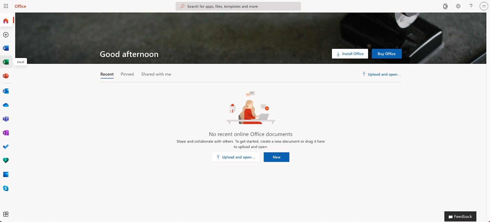
The easiest way to get started with Excel, is to use Office 365.
Office 365 does not require downloading and installation of the program. It simply runs in your browser.
In our tutorial we will use Office 365, which can be accessed from .
Install
Once you have successfully logged into Office through ,
click on the Excel icon on the left side to enter the application:
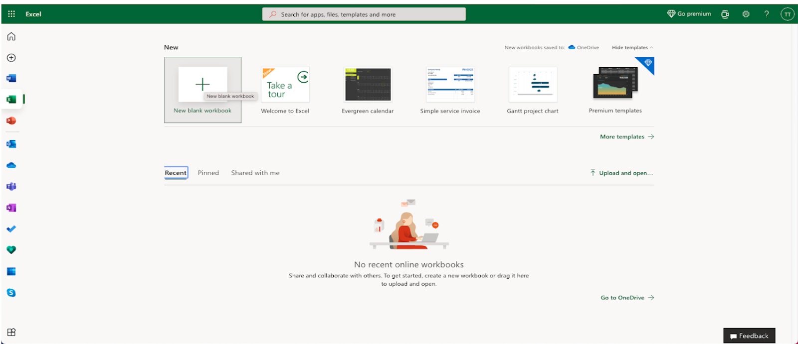
After entering the Excel application, click on the New blank workbook button to get started with a new workbook.
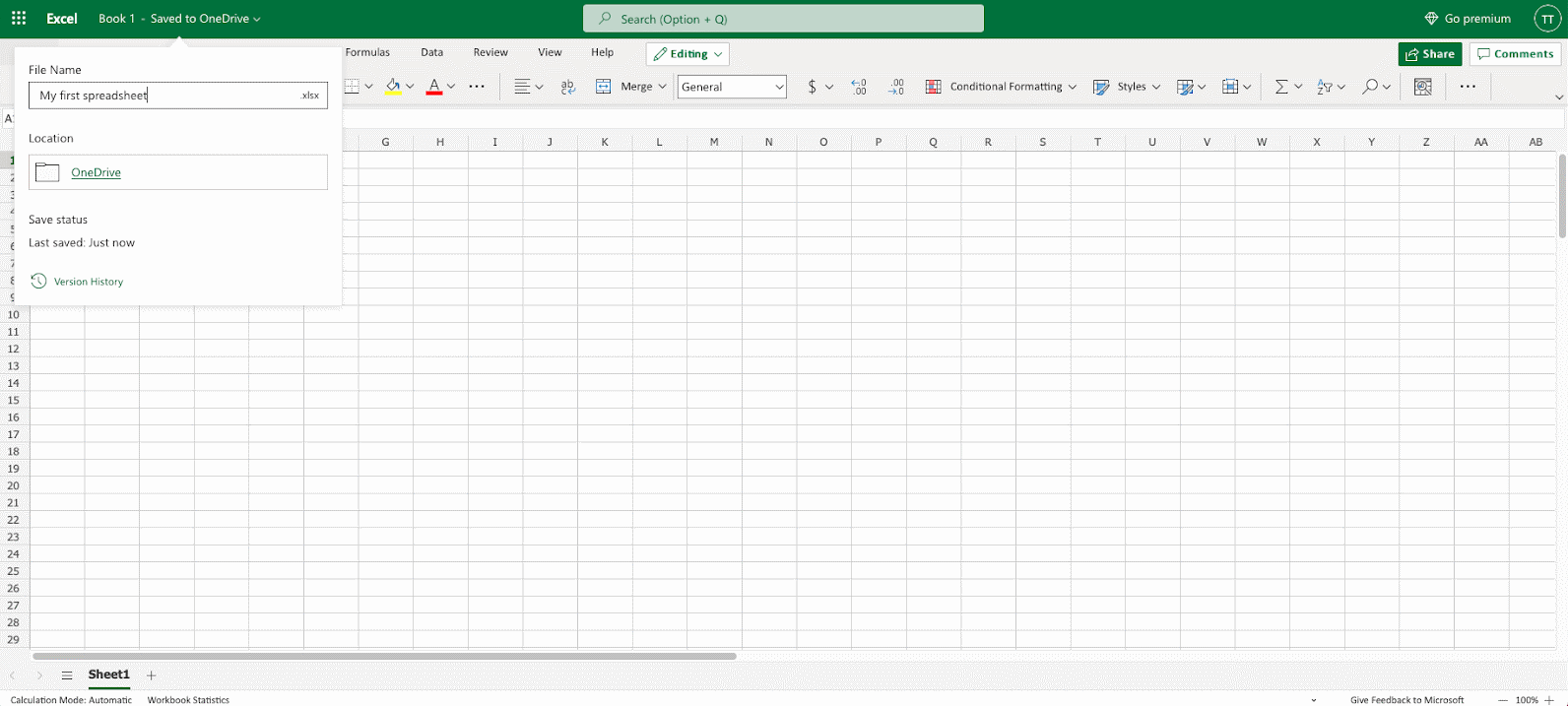
Enter a name for your workbook, and hit the enter button:
The Excel view has columns and rows, similar to a squared math exercise book.
Do not worry if the functionality looks overwhelming at first. You will get comfortable as you learn more in the chapters to come.
For now focus on the rows, columns, and the cells.
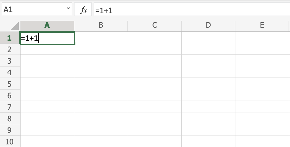
Ok. Let's make a function!
First, double click the cell A1, the one that is marked with the green rectangle in the picture.
Second, type =1+1.
Third, hit the enter button:
Congratulations! You have typed your first function,
1+1=2.
Excel Overview
Overview
This chapter is about giving you an overview of Excel. Excel's structure is made of two pieces, the Ribbon and the Sheet.
Have a look at the picture below. The Ribbon is marked with a red rectangle and the
Sheet is marked with a yellow rectangle:
First, let's start with explaining the Ribbon.
The Ribbon explained
The Ribbon provides shortcuts to Excel commands. A command is an action that allows you to make something happen. This can for example be to: insert a table, change the font size, or to change the color of a cell.
The Ribbon may look crowded and hard to understand at first. Don't be scared, It will become easier to navigate and use as you learn more. Most of the time we tend to use the same functionalities over again.
The Ribbon is made up by the App launcher, Tabs, Groups and Commands. In this section we will explain the different parts of the
Ribbon.
App launcher
The App launcher icon has nine dots and is called the Office 365 navigation bar. It allows you to access the different parts of the Office 365 suite, such as Word, PowerPoint and Outlook. App launcher can be used to switch seamlessly between the Office 365 applications.
Tabs
The tab is a menu with sub divisions sorted into groups. The tabs allow users to quickly navigate between options of menus which display different groups of functionality.
Groups
The groups are sets of related commands. The groups are separated by the thin vertical line break.
Commands
The commands are the buttons that you use to do actions.
Now, let's have a look at the Sheet. Soon you will be able to understand the relationship between the
Ribbon and the Sheet, and you can make things happen.
The Sheet explained
The Sheet is a set of rows and columns. It forms the same pattern as we have in math exercise books, the rectangle boxes formed by the pattern are called cells.
Values can be typed to cells.
Values can be both numbers and letters:
Each cell has its unique reference, which is its coordinates, this is where the columns and rows intersect.
Let's break this up and explain by an example
Have a look at the picture below. Hello world was typed in cell C4. The reference can be found by clicking on the relevant cell and seeing the reference in the
Name Box to the left, which tells you that the cell's reference is C4.
Another way to find the reference is to first find the column, in this case C, then map that towards the row, in this case 4, which gives us the reference of C4.
Note: The reference of the cell is its coordinates. For example, C4 has the coordinates of column C and row 4. You find the cell in the intersection of the two. The letter is always the column and the number is always the row.
Multiple Sheets
You start with one Sheet by default when you create a new workbook. You can have many sheets in a workbook. New sheets can be added and removed. Sheets can be named to making it easier to work with data sets.
Are you up for the challenge? Let's create two new sheets and give them useful names.
First, click the plus icon, shown in the picture below, create two new sheets:
Tip: You can use the hotkey Shift + F11 to create new sheets. Try it!
Second, right click with your mouse on the relevant sheet and click rename:
Third, enter useful names for the three sheets:
In this example we used the names Data Visualization, Data Structure and Raw Data. This is a typical structure when you are working with data.
Good job! You have now created your first workbook with three named sheets!
Chapter Summary
The workbook has two main components: the Ribbon and the
Sheet.
The Ribbon is used to navigate and access commands.
The Sheet is made up of columns and rows, which make cells.
Each cell has its unique reference. You can add new sheets to your workbook and name them.
In the next chapters you will learn more about the sheet, formulas, ranges and functions.
Excel Syntax
Syntax
A formula in Excel is used to do mathematical calculations. Formulas always start with the equal sign = typed in the cell, followed by your calculation.
Note: You claim the cell by selecting it and typing the equal sign (=)
Creating formulas, step by step
Select a cell
Type the equal sign (=)
Select a cell or type value
Enter an arithmetic operator
Select another cell or type value
Press enter
For example =1+1 is the formula to calculate 1+1=2
Note: The value of a cell is communicated by reference(value) for example A1(2)
Using Formulas with Cells
You can type values to cells and use them in your formulas.
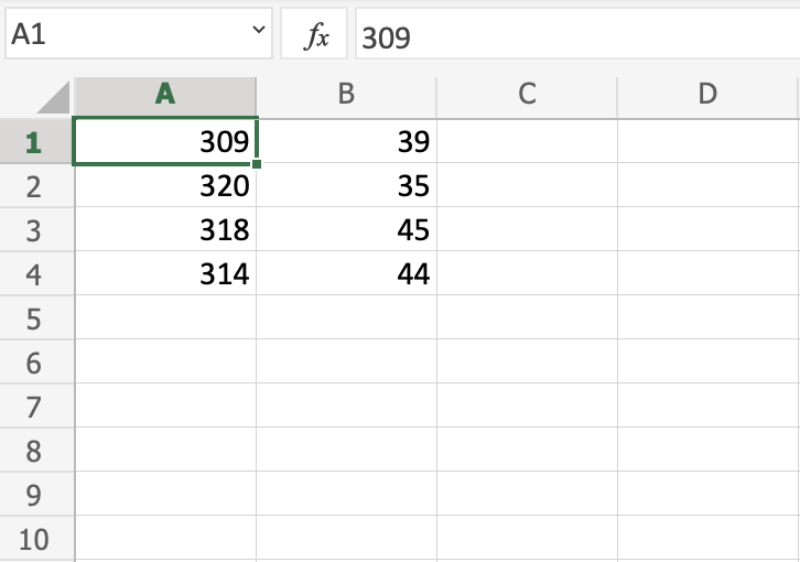
Lets type some dummy values to get started. Double click the cells to type values into them. Go ahead and type:
A1(309)
A2(320)
B1(39)
B2(35)
Compare with the picture shown below:
Note: Type values by selecting a cell, claim it by entering the equal sign (=)
and then type your value. For example =309.
Well done! You have successfully typed values to cells and now we can use them to create formulas.
Here is how to do it, step by step.
Select the cell C1
Type the equal sign (=)
Left click on A1, the cell that has the (309) value
Type the minus sign (-)
Left click on B2, the cell that has the (35) value
Hit enter
Tip: The formula can be typed directly without clicking the cells. The typed formula would be the same as the value in C1(=A1-B2).
The result after hitting the enter button is C1(274). Did you make it?
Another Example
Let's try one more example, this time let's make the formula =A2-B1.
Here is how to do it, step by step.
Select the cell C2
Type the equal sign (=)
Left click A2, the cell that has the (320) value
Type the minus sign (-)
Left click B1, the cell that has the (39) value
Hit the enter button
You got the result C2(281), right? Way to go!
Note: You can make formulas with all four arithmetic operations, such as addition (+), subtraction (-), multiplication (*) and division (/).
Here are some examples:
=2+4 gives you 6
=4-2 gives you 2
=2*4 gives you 8
=2/4 gives you 0.5
In the next chapter you will learn about Ranges and how data
can be moved in the Sheet.
Ranges
Range is an important part of Excel because it allows you to work with selections of cells.
There are four different operations for selection;
Selecting a cell
Selecting multiple cells
Selecting a column
Selecting a row
Before having a look at the different operations for selection, we will introduce the Name Box.
The Name Box
The Name Box shows you the reference of which cell or range you have selected. It can also be used to select cells or ranges by typing their values.
You will learn more about the Name Box later in this chapter.
Selecting a Cell
Cells are selected by clicking them with the left mouse button or by navigating to them with the keyboard arrows.
It is easiest to use the mouse to select cells.
To select cell A1, click on it:
Selecting Multiple Cells
More than one cell can be selected by pressing and holding down CTRL or Command and left clicking the cells. Once finished with selecting, you can let go of CTRL or Command.
Lets try an example: Select the cells A1, A7, C1, C7 and B4.
Did it look like the picture below?
Selecting a Column
Columns are selected by left clicking it. This will select all cells in the sheet related to the column.
To select column A, click on the letter A in the column bar:
Selecting a Row
Rows are selected by left clicking it. This will select all the cells in the sheet related to that row.
To select row 1, click on its number in the row bar:
Selecting the Entire Sheet
The entire spreadsheet can be selected by clicking the triangle in the top-left corner of the spreadsheet:
Now, the whole spreadsheet is selected:
Note: You can also select the entire spreadsheet by pressing Ctrl+A for Windows, or Cmd+A for MacOS.
Selection of Ranges
Selection of cell ranges has many use areas and it is one of the most important concepts of Excel. Do not think too much about how it is used with values. You will learn about this in a later chapter. For now let's focus on how to select ranges.
There are two ways to select a range of cells
Name Box
Drag to mark a range.
The easiest way is drag and mark. Let's keep it simple and start there.
How to drag and mark a range, step-by-step:
Select a cell
Left click it and hold the mouse button down
Move your mouse pointer over the range that you want selected. The range that is marked will turn grey.
Let go of the mouse button when you have marked the range
Let's have a look at an example for how to mark the range A1:E10.
Note: You will learn about why the range is called A1:E10 after this example.
Select cell A1:
Press and hold A1 with the left mouse button. Move to the mouse pointer to mark the selection range. The grey area helps us to see the covered range.
Let go of the left mouse button when you have marked the range A1:E10:
You have successfully selected the range A1:E10. Well done!
The second way to select a range is to enter the range values in the Name Box. The range is set by first entering the cell reference for the top left corner, then the bottom right corner. The range is made using those two as coordinates. That is why the cell range has the reference of two cells and the : in between.
Top left corner reference : Right bottom corner reference
The range shown in the picture has the value of A1:E10:
The best way for now is to use the drag and mark method as it is easier and more visual.
In the next chapter you will learn about filling and how this applies to the ranges that we have just learned.
Filling
Filling makes your life easier and is used to fill ranges with values, so that you do not have to type manual entries.
Filling can be used for:
Copying
Sequences
Dates
Functions (*)
For now, do not think of functions. We will cover that in a later chapter.
How To Fill
Filling is done by selecting a cell, clicking the fill icon and selecting the range using drag and mark while holding the left mouse button down.
The fill icon is found in the bottom right corner of the cell and has the icon of a small square. Once you hover over it your mouse pointer will change its icon to a thin cross.
Click the fill icon and hold down the left mouse button, drag and mark the range that you want to cover.
In this example, cell A1 was selected and the range A1:A10 was marked.
Now that we have learned how to fill. Let's look into how to copy with the fill function.
Fill Copies
Filling can be used for copying. It can be used for both numbers and words.
Let's have a look at numbers first.
In this example we have typed the value A1(1):
Filling the range A1:A10 creates ten copies of 1:
The same principle goes for text.
In this example we have typed A1(Hello World).
Filling the range A1:A10 creates ten copies of "Hello World":
Now you have learned how to fill and to use it for copying both numbers and words. Let's have a look at sequences.
Fill Sequences
Filling can be used to create sequences. A sequence is an order or a pattern. We can use the filling function to continue the order that has been set.
Sequences can for example be used on numbers and dates.
Let's start with learning how to count from 1 to 10.
This is different from the last example because this time we do not want to copy, but to count from 1 to 10.
Start with typing A1(1):
First we will show an example which does not work, then we will do a working one. Ready?
Lets type the value (1) into the cell A2, which is what we have in A1. Now we have the same values in both A1 and A2.
Let's use the fill function from A1:A10 to see what happens. Remember to mark both values before you fill the range.
What happened is that we got the same values as we did with copying. This is because the fill function assumes that we want to create copies as we had two of the same values in both the cells A1(1) and A2(1).
Change the value of A2(1) to A2(2). We now have two different values in the cells A1(1) and A2(2). Now, fill A1:A10 again. Remember to mark both the values (holding down shift) before you fill the range:
Congratulations! You have now counted from 1 to 10.
The fill function understands the pattern typed in the cells and continues it for us.
That is why it created copies when we had entered the value (1) in both cells, as it saw no pattern. When we entered (1) and (2) in the cells it was able to understand the pattern and that the next cell A3 should be (3).
Let's create another sequence. Type A1(2) and A2(4):
Now, fill A1:A10:
It counts from 2 to 20 in the range A1:A10.
This is because we created an order with A1(2) and A2(4).
Then it fills the next cells, A3(6), A4(8), A5(10) and so on. The fill function understands the pattern and helps us continue it.
Sequence of Dates
The fill function can also be used to fill dates.
Note: The date format depends on you regional language settings.
For example 14.03.2023 vs. 3/14/2023.
Test it by typing A1(29.07.2021):
And fill the range A1:A10:
The fill function has filled 10 days from A1(29.07.2021) to A10(07.08.2021).
Note that it switched from July to August in cell A4. It knows the calendar and will count real dates.
Combining Words and Letters
Words and letters can also be combined.
Type A1(Hello 1) and A2(Hello 2):
Next, fill A1:A10 to see what happens:
The result is that it counts from A1(Hello 1) to A10(Hello 10). Only the numbers have changed.
It recognised the pattern of the numbers and continued it for us. Words and numbers can be combined, as long as you use a recognizable pattern for the numbers.
Double Click to Fill
The fill function can be double clicked to complete formulas in a range:
Note: For the double click to work it has to see a recognizable pattern.
For example: by using headers, or with the formulas in the columns or rows next to the data.
Double Click to Fill Example
Let's use the Double click fill function to calculate the AttackB2:B20 + Defense C2:C20 for the Pokemons in the range D2:D20.
Select D2
Type =
Select B2
Type +
Select C2
Hit enter
Double click the fill function
Way to go! The function understands the pattern and completes the calculation for D2:D20. Note that it stops when there is no more data to calculate, at row 20.
A Non-Working Example
Delete values in the range D1:D20
Enter the formula "=B2+C2" in E2
Note: There is no header for Columns D and E. There are blank cells in between.
Double click the fill function.
Waiting...
The fill function is just loading without filling the rows. It is not understanding the pattern.
Give it more clues.
Add a header to see what happens. Enter "Atk+def" in E1
Double click the fill function.
Loading... Still nothing...
One more header. Enter "Random" in D1
Double click the fill function.
Is the gap closed?
There we go! The function recognised the pattern and filled in the formulas for each row.
Adding headers helped the function to understand the relationship between the data.
Excel Move Cells
Moving Cells
There are two ways to move cells: Drag and drop or by copy and paste.
Drag and Drop
Let's start by typing or copying some values that we can work with:
Next, start by marking the area A1:B4:
You can drag and drop the range by pressing and holding the left mouse button on the border. The mouse cursor will change to the move symbol when you hover over the border.
Drag and drop it when you see the symbol.
Move the range to B2:C5 as shown in the picture:
Great! Now you have created more space, so that we have room for more data.
Note: It is important to give context to the data, making the spreadsheet easy to understand. This can be done by adding text which explains the data.
Let's go ahead and give the data more context. Type or copy the following values:
Yes, that is right, we are looking at Pokemons! Giving context to the data is always helpful.
Next, lets see how we can move data by using cut and paste.
Cut and Paste
Ranges can be moved by cutting and pasting values from one place to another.
Tip: You can cut using the hotkey CTRL+X and paste by CTRL+V. This saves you time.
Mark the range A1:C5
Right click the marked area, and click on the "Cut" command, which has scissors as its icon:
Cutting makes the range white-grey with dotted borders. This indicates that the range is cutted and ready for pasting.
Right click the paste destination B6 and left click the paste icon.
You have successfully cutted and pasted the range from A1:C5 to B6:D10.
Copy and paste
Copy and paste works in the same way as cut and paste. The difference is that it does not remove the original cells.
Let's copy the cells back from B6:D10 to A1:C5.
Tip: You can copy using the hotkey CTRL+C and paste by CTRL+V. This saves you time. Try it!
Mark the range B6:D10.
Right click the marked area, and click on the "Copy" command which has two papers as its icon.
Copying gives the range a dotted green border. This indicates that the range is copied and ready for pasting.
Right click the paste destination A1 and left click the paste icon:
The difference between cutting and copying, is that cutting removes the originals, while copying leaves the originals.
Next, let's delete the original data and keep the data in the A1:C5 range.
Delete Data
Select the original cells and remove them by pressing the "Delete" button on the keyboard:
Excel Add Cells
Adding New Columns
Columns can be added and deleted. You access the menu by right clicking the column letter. New columns are added to the same place you clicked.
Let's try to create a new column B.
Right click on the column and select "Insert Columns":
And a new column is created:
Next, we need to get some Pokemon trainers in there. Type or copy the following data in the new column B:
Adding New Rows
Rows can also be added and deleted. You access the menu by right clicking the row number. New rows are added to the same place you clicked.
Let's try to create a new row 4.
We forgot to add Iva's Pokemon, Marowak. Lets add his data to the new row 4, by typing or copying the following values:
Excellent job!
Delete Cells
Cells can be deleted by selecting them, and pressing the delete button.
Note: The delete function will not delete the formatting of the cell, just the value inside of it.
Let's have a look at three examples.
Example 1
Pressing the delete button:
Example 2
Pressing the delete button:
Example 3
With formatting:
Pressing the delete button:
Note that it only deletes the value in the cells, and not the formatting (the color).
Note: You will learn more about formatting, and how to style cells in a later chapter.
Undo
The Undo function lets you reverse an action.
Undo is helpful if you regret an action and want to go back to how it was before.
Examples of use
Undo deleting a formula
Undo adding a column
Undo removing a row
Note: You cannot Undo things that you do in the File Menu, such as deleting a sheet, saving a spreadsheet or changing the options. The thumb rule is that you can Undo things you do in your sheet.
There are two ways to access the Undo command.
1) Pressing the Undo button in the Ribbon:
2) Using the keyboard shortcut CTRL + Z / Command + Z
Let's have a look at an example:
Note: It is recommended to practice using the keyboard shortcut. It saves you time!
Redo
The Redo function has the opposite effect as Undo, it reverses the Undo action.
Redo is helpful if you regret using Undo.
Note: The Redo command is only available if you have used Undo.
There are two ways to access the Redo command.
1) Pressing the Redo button in the Ribbon:
2) Using the keyboard shortcut CTRL + Y / Command + Y
Tip: Practice for yourself to get familiar with Undo and Redo.
Excel Formulas
Formulas
A formula in Excel is used to do mathematical calculations. Formulas always start with the equal sign (=) typed in the cell, followed by your calculation.
Formulas can be used for calculations such as:
=1+1
=2*2
=4/2=2
It can also be used to calculate values using cells as input.
Let's have a look at an example.
Type or copy the following values:
Now we want to do a calculation with those values.
Step by step:
Select C1 and type (=)
Left click A1
Type (+)
Left click A2
Press enter
You got it! You have successfully calculated A1(2) + A2(4) = C1(6).
Note: Using cells to make calculations is an important part of Excel and you will use this alot as you learn.
Lets change from addition to multiplication, by replacing the (+) with a (*). It should now be =A1*A2, press enter to see what happens.
You got C1(8), right? Well done!
Excel is great in this way. It allows you to add values to cells and make you do calculations on them.
Now, try to change the multiplication (*) to subtraction (-) and dividing (/).
Delete all values in the sheet after you have tried the different combinations.
Let's add new data for the next example, where we will help the Pokemon trainers to count their Pokeballs.
Type or copy the following values:
The data explained:
Column A: Pokemon Trainers
Row 1: Types of Pokeballs
Range B2:D4: Amount of Pokeballs, Great balls and Ultra balls
Note: It is important to practice reading data to understand its context. In this example you should focus on the trainers and their Pokeballs, which have three different types: Pokeball, Great ball and Ultra ball.
Let's help Iva to count her Pokeballs. You find Iva in A2(Iva). The values in row 2 B2(2), C2(3), D2(1) belong to her.
Count the Pokeballs, step by step:
Select cell E2 and type (=)
Left click B2
Type (+)
Left click C2
Type (+)
Left click D2
Hit enter
Did you get the value E2(6)? Good job! You have helped Iva to count her Pokeballs.
Now, let's help Liam and Adora with counting theirs.
Do you remember the that we learned about earlier? It can be used to continue calculations sidewards, downwards and upwards. Let's try it!
Lets use the fill function to continue the formula, step by step:
Select E2
Fill E2:E4
That is cool, right? The fill function continued the calculation that you used for Iva and was able to understand that you wanted to count the cells in the next rows as well.
Now we have counted the Pokeballs for all three; Iva(6), Liam(12) and Adora(15).
Let's see how many Pokeballs Iva, Liam and Adora have in total.
The total is called SUM in Excel.
There are two ways to calculate the SUM.
Adding cells
SUM function
Excel has many pre-made functions available for you to use. The SUM
function is one of the most used ones. You will learn more about functions in a later chapter.
Let's try both approaches.
Note: You can navigate to the cells with your keyboard arrows instead of left clicking them. Try it!
Sum by adding cells, step by step:
Select cell E5, and type =
Left click E2
Type (+)
Left click E3
Type (+)
Left click E4
Hit enter
The result is E5(33).
Let's try the SUM function.
Remember to delete the values that you currently have in E5.
SUM function, step by step:
Type E5(=)
Write SUM
Double click SUM in the menu
Mark the range E2:E4
Hit enter
Great job! You have successfully calculated the SUM using the SUM function.
Iva, Liam and Adora have 33 Pokeballs in total.
Let's change a value to see what happens. Type B2(7):
The value in cell B2 was changed from 2 to 7. Notice that the formulas are doing calculations when we change the value in the cells, and the SUM is updated from 33 to 38. It allows us to change values that are used by the formulas, and the calculations remain.
Chapter Summary
Values used in formulas can be typed directly and by using cells. The formula updates the result if you change the value of cells, which is used in the formula. The fill function can be used to continue your formulas upwards, downwards and sidewards. Excel has pre-built functions, such as SUM.
In the next chapter you will learn about relative and absolute references.
Excel Relative References
Relative and Absolute References
Cells in Excel have unique references, which is its location.
References are used in formulas to do calculations, and the fill function can be used to continue formulas sidewards, downwards and upwards.
Excel has two types of references:
Relative references
Absolute references
Absolute reference is a choice we make. It is a command which tells Excel to lock a reference.
The dollar sign ($) is used to make references absolute.
Example of relative reference: A1
Example of absolute reference: $A$1
Relative reference
References are relative by default, and are without dollar sign ($).
The relative reference makes the cells reference free. It gives the fill function freedom to continue the order without restrictions.
Let's have a look at a relative reference example, helping the Pokemon trainers to count their Pokeballs (B2:B7) and Great balls (C2:C7).
The result is: D2(5):
Next, fill the range D2:D7:
The references being relative allows the fill function to continue the formula for rows downwards.
Have a look at the formulas in D2:D7. Notice that it calculates the next row as you fill.
A Non-Working Example
Let's try an example that will not work.
Fill D2:G2, filling to the right instead of downwards. Resulting in strange numbers:
Have a look at the formulas.
It assumes that we are calculating sidewards and not downwards.
The numbers that we want to calculate need to be in the same direction as we fill.
Excel Absolute References
Absolute References
Absolute reference is when a reference has the dollar sign ($).
It locks a reference in the formula.
Add $ to the formula to use absolute references.
The dollar sign has three different states:
Absolute for column and row. The reference is absolutely locked.
Example =$A$1
Absolute for the column. The reference is locked to that column. The row remains relative.
Example =$A1
Absolute for the row. The reference is locked to that row. The column remains relative.
Example =A$1
Let's have a look at an example helping the Pokemon trainers to calculate prices for Pokeballs
Type or copy the following data:
Data explained
There are 6 trainers: Iva, Liam, Adora, Jenny, Iben and Kasper.
They have different amount of Pokeballs each in their shop cart
The price per Pokeball is 2 coins
Help them to calculate the prices for the Pokeballs.
The price's reference is B11, we do not want the fill function to change this, so we lock it.
The reference is absolutely locked by using the formula $B$11.
How to do it, step by step:
Type C2(=)
Select B11
Type ($) before the B and 11 ($B$11)
Type (*)
Select B2
Hit enter
Auto fill C2:C7
Congratulations! You successfully calculated the prices for the Pokeballs using an absolute reference.
Addition Operator
Addition uses the + symbol in Excel, and is also known as plus.
There are two ways to do addition in Excel. Either by using the + symbol in a formula or by using the SUM function.
How to add cells:
Select a cell and type (=)
Select a cell
Type (+)
Select another cell
Hit enter
You can add more cells to the formula by typing (+) between the cells.
Let's have a look at some examples.
Adding Two Manual Entries
Type A1(=)
Type 5+5
Hit enter
Congratulations! You have successfully added 5+5=10.
Adding Two Cells
First let's add some numbers to work with. Type the following values:
How to do it, step by step:
Type B1(=)
Select A1
Type (+)
Select A2
Hit enter
Great!30 is the result by adding A1 and A2.
Adding Several Cells
First let's add some numbers to work with. Type the following values:
Step by step to add several cells:
Type B1(=)
Select A1
Type (+)
Select A2
Type (+)
Select A3
Type (+)
Select A4
Type (+)
Select A5
Hit enter
Good job! You have successfully added five cells!
Adding with SUM
Let's keep the numbers from the last exercise. If you did last exercise, remove the value in B1.
Step by step to add with SUM:
Type B1(=SUM)
Double click the SUM command
Mark the range A1:A5
Hit enter
Note:SUM saves you time! Keep practicing this function.
Adding Using Absolute Reference
You can also lock a cell and add it to other cells.
How to do it, step by step:
Select a cell and type (=)
Select the cell you want to lock, add two dollar signs ($) before the column and row
Type (+)
Fill a range
Let's have a look at an example where we add B(5) to the range A1:A10 using absolute reference and the fill function.
Type the values:
Step by step:
Type C1(=)
Select B1
Type dollar sign before column and row $B$1
Type (+)
Select A1
Hit enter
Fill the range C1:C10
Great! You have successfully used absolute reference to add B1(5) with the range A1:A10.
Subtraction Operator
Subtraction uses the - symbol, and is also known as minus.
How to subtract cells:
Select a cell and type (=)
Select the minuend
Type (-)
Select the subtrahend
Hit enter
Note: The minuend is the number to which the subtrahend subtracts from.
You can add more cells to the formula by typing (-) between the cells.
Let's have a look at some examples.
Subtracting Two Manual Entries
Let's start with adding in a formula. Start with a clean sheet
Step by step:
Type A1(=)
Type 100-50
Hit enter
Tip: You can add more values into the formula by typing (-) between the cells.
Subtracting Using Two Cells
Let's add some numbers to work with. Type the following values:
Subtracting using two cells, step by step:
Type A3(=)
Select A1
Type (-)
Select A2
Hit enter
Subtracting Using Many Cells
Let's subtract using many cells. First, type the following values:
Step by step:
Type B1(=)
Select A1
Type (-)
Select A2
Type (-)
Select A3
Type (-)
Select A4
Type (-)
Select A5
Hit enter
Subtracting Using Absolute Reference
You can lock a cell and subtract it from other cells.
How to do it, step by step:
Select a cell and type (=)
Select the minuend
Type (-)
Select the subtrahend and add two dollar signs ($) before the column and row
Hit enter
Fill the range
Note: The minuend is the number to which the subtrahend subtracts from.
Let's have a look at an example where we subtract B(5) from the range A1:A10 using absolute reference and fill function.
Type the values:
Step by step:
Type C1(=)
Select A1
Type (-)
Select B1 and type dollar sign before column and row $B$1
Hit enter
Fill C1:C10
You got it! You have successfully used absolute reference to subtract B1(5) from the minuend range A1:A10.
Multiplication Operator
Multiplication uses the * symbol in Excel.
How to multiply cells:
Select a cell and type (=)
Select a cell
Type (*)
Select another cell
Hit enter
You can add more cells to formula by typing (*) between the cells.
Let's have a look at some examples.
Multiplying Manual Entries
Let's start with adding in a formula. Start with a clean sheet.
Step by step:
Type A1(=)
Type 2*2
Hit enter
Multiplying Two Cells
Let's add some numbers to work with. Type the following values:
Step by step:
Type A3(=)
Select A1
Type (*)
Select A2
Hit enter
Multiplying Using Absolute Reference
You can lock a cell and multiply it with other cells.
How to do it, step by step:
Select a cell and type (=)
Select the cell you want to lock and add two dollar signs ($) before the column and row
Type (*)
Select another cell
Hit enter
Fill the range
Let's have a look at an example where we multiply B(5) with the range A1:A10 using absolute reference and the fill function.
Type the values:
Step by step:
Type C1(=)
Select B1 type dollar sign before column and row $B$1
Type (*)
Select A1
Hit enter
Fill C1:C10
You got it! You have successfully used absolute reference to multiply B1(5) with the range A1:A10.
Division Operator
Division uses the / symbol in Excel.
How to do division cells:
Select a cell and type (=)
Select a cell
Type (/)
Select another cell
Hit enter
You can add more cells to the formula by typing (/) between the cells.
Let's have a look at some examples.
Dividing Manual Entries
Let's start with adding in a formula. Start with a clean sheet.
Step by step:
Type A1(=)
Type 4/2
Hit enter
Dividing Two Cells
Let's add some numbers to work with. Type the following values:
Step by step:
Type A3(=)
Select A1
Type (/)
Select A2
Hit enter
Dividing Using Absolute Reference
You can lock a cell and divide it with other cells.
How to do it, step by step:
Select a cell and type (=)
Select the dividend
Type (/)
Select the divisor lock and add two dollar signs ($) before the column and row
Hit enter
Fill the range
Note: Dividend is the number being divided by the divisor.
Let's have a look at an example where we divide B(5) with the range A1:A10 using absolute reference and fill function.
Type the values:
Step by step:
Type C1(=)
Select A1
Type (/)
Select B1 type dollar sign before column and row $B$1
Hit enter
Fill C1:C10
Goob job! You have successfully used absolute reference to divide B1(5) with the range A1:A10.
Parentheses
Parentheses () is used to change the order of an operation.
Using parentheses makes Excel do the calculation for the numbers inside the parentheses first, before calculating the rest of the formula.
Parentheses are added by typing () on both sides of numbers, like (1+2).
Examples
No parentheses
=10+5*2
The result is 20 because it calculates (10+10)
With parentheses
=(10+5)*2
The result is 30 because it calculates (15)*2
Formulas can have groups of parentheses.
=(10+5)+(2*4)+(4/2)
Note: Cells can be used as values in the formulas inside parentheses, like =(A1+A2)*B5. We have used manual entries in our examples to keep things simple.
Let's have a look at some real examples in Excel.
Without Parentheses
The result is 17, the calculation is 2+15. It uses 15 because 3*5=15.
With One Parentheses
The result is 25, the calculation is 5*5. It uses 5 because it has calculated numbers inside the parentheses (2+3)=5 first.
With Many Parentheses
The result is 17, the calculation is 5+8+4. The numbers inside the parentheses are calculated first.
Nesting Parentheses
When using more advanced formulas you may need to nest parentheses. You can look at this like an onion, which has many layers. Excel will calculate the numbers inside the parentheses first, layer by layer, starting with the inner layer.
Example no nesting
=2*2+3*4+5*5*2
It calculates the values flat as you would do with a calculator.
Example nesting
=((2*2)+(3*4)+(5*5))*2
Let's break it down and explain.
Nesting creates layers like an onion. You can have many layers. This example uses two, the inner and outer layers.
It starts with calculating the numbers in the inner layer:
=((2*2)+(3*4)+(5*5))*2
=((4)+(12)+25))*2 Calculates the inner layer
=(41)*2 Calculates the outer layer
82
Chapter Summary
Parentheses can be used to change the order of an operation. The numbers inside the parentheses gets calculated first. A formula can have sets of parentheses. More advanced formulas can use nesting to create layers of operations, like an onion. It calculates the inner layer first, then the next, and so on.
Functions
Excel has many premade formulas, called functions.
Functions are typed by = and the functions name.
For example =SUM
Once you have typed the function name you need to apply it to a range.
For example =SUM(A1:A5)
The range is always inside of parentheses.
Function
Description
=AND
Returns TRUE or FALSE based on two or more conditions
=AVERAGE
Calculates the average (arithmetic mean)
=AVERAGEIF
Calculates the average of a range based on a TRUE or FALSE condition
=AVERAGEIFS
Calculates the average of a range based on one or more TRUE/FALSE conditions
=CONCAT
Links together the content of multiple cells
=COUNT
Counts cells with numbers in a range
=COUNTA
Counts all cells in a range that has values, both numbers and letters
=COUNTBLANK
Counts blank cells in a range
=COUNTIF
Counts cells as specified
=COUNTIFS
Counts cells in a range based on one or more TRUE or FALSE condition
=IF
Returns values based on a TRUE or FALSE condition
=IFS
Returns values based on one or more TRUE or FALSE conditions
=LEFT
Returns values from the left side of a cell
=LOWER
Reformats content to lowercase
=MAX
Returns the highest value in a range
=MEDIAN
Returns the middle value in the data
=MIN
Returns the lowest value in a range
=MODE
Finds the number seen most times. The function always returns a single number
=NPV
The NPV function is used to calculate the Net Present Value (NPV)
=OR
Returns TRUE or FALSE based on two or more conditions
=RAND
Generates a random number
=RIGHT
Returns values from the right side of a cell
=STDEV.P
Calculates the Standard Deviation (Std) for the entire population
=STDEV.S
Calculates the Standard Deviation (Std) for a sample
=SUM
Adds together numbers in a range
=SUMIF
Calculates the sum of values in a range based on a TRUE or FALSE condition
=SUMIFS
Calculates the sum of a range based on one or more TRUE or FALSE condition
=TRIM
Removes irregular spacing, leaving one space between each value
=VLOOKUP
Allows vertical searches for values in a table
=XOR
Returns TRUE or FALSE based on two or more conditions
Formatting
Excel has many ways to format and style a spreadsheet.
Why format and style your spreadsheet?
Make it easier to read and understand
Make it more delicate
Styling is about changing the looks of cells, such as changing colors, font, font sizes, borders, number formats, and so on.
The most used styling functions are:
Colors
Fonts
Borders
Number formats
Grids
There are two ways to access the styling commands in Excel:
The Ribbon
Formatting menu, by right clicking cells
Read more about the Ribbon in the Excel overview chapter.
Styling Commands in Ribbon
The Ribbon can be expanded by clicking the arrow/caret-down icon on the right side. This gives access to more commands:
Styling Commands, Right Clicking Cells
You can also right-click on any cell to style it:
Styling commands can be accessed from both views.
Chapter summary
Formatting is used to make spreadsheets more readable. There are many ways to add styles. The most common ones are; Color, Font, Number format and Grids.
Format Painter
The format painter is a command which lets you copy formatting from one cell to another.
It is a great tool, which saves you lots of time!
The Format painter can be used to copy to single cells or ranges.
Format Painter is used by clicking on its button in the Ribbon, found in the Clipboard group.
How To Use the Format Painter
Select the cell that you want to copy
Click the Format Painter button
Select a cell or range
Let's try some examples and copy formats with Colors and font Characteristics, such as bold, italic and underline:
Copy the red color from A1 to B1.
Step by step:
Select A1
Click the Format Painter button
Select B1
Notice the dotted border around A1. This indicates that the format is copied and ready for pasting. Let's paste it to B1!
Great job!
Copy and Paste Color to Multiple Cells
Copy B2 to C2. That is right, let's try to paste to a range of two cells!
Select A2
Click the Format Painter button
Select B2 and hold an drag to C2
That's the way! The format painter can be used for single cells and on ranges.
Copy Font Characteristics
Last example. Copy the Font Characteristics from A4:A6 to B4:B6.
Step by step:
Mark A4:A6
Click the Format Painter button
Drag and mark B4:B6
Good job!
Colors
Colors are specified by selection or by using Hexadecimal and RGB codes.
Tip: You can learn more about colors in our HTML/CSS Colors Tutorial.
Theme and Standard Colors
Excel has a set of themes and standard colors available for use. You select a color by clicking it:
The "More Colors" option allows you to select custom colors by entering a RGB or HEX code.
Hexadecimal Colors
Excel supports Hexadecimal color values
A hexadecimal color is specified with: #RRGGBB.
RR (red), GG (green) and BB (blue) are hexadecimal integers between 00 and FF specifying the intensity of the color.
For example, #0000FF is displayed as blue, because the blue component is set to its highest value (FF) and the others are set to 00.
RGB Colors
Excel supports RGB color values.
An RGB color value is specified with: rgb( RED , GREEN , BLUE ).
Each parameter defines the intensity of the color as an integer between 0 and 255.
For example, rgb(0,0,255) is rendered as blue, because the blue parameter is set to its highest value (255) and the others are set to 0.
Tip: Try W3schools.com color picker to find your color! https://www.w3schools.com/colors/colors_picker.asp
Applying colors
Colors can be applied to cells, text and borders.
Colors are applied to cells by using the "Fill color" function.
How to apply colors to cells:
Select color
Select range
Click the Fill Color button
The "Fill color" button remembers the color you used the last time.
Color options are explored by clicking on the arrow-down icon (), next to the Fill color command:
The option allows selection of theme colors, standard colors or use of HEX or RGB codes by clicking on the More Colors option:
Colors are made from red, green, blue and are universal. Entering a color in one way will give you the code in the other. For example if you enter a HEX code, it will give you the RGB code for the same color.
Let's try some examples.
Starting with theme and standard colors:
Great!
Try to apply the following colors:
Theme color blue (accent 5) to A3:F3.
Theme color green (accent 6) and A5:F5.
Did you make it?
Let's apply colors using HEX and RGB codes.
Apply HEX code #ffcb05 to A7:F7:
Step by step:
Select A7:F7
Open color options
Click More colors
Insert #ffcb05 in the HEX input field
Hit enter
Notice that applying the HEX code gives the RGB code for the same color, and shows where that color is positioned on the color map.
Apply RGB code 60, 90, 166 to A9:F9
Step by step:
Select A9:F9
Open color options
Click More colors
Insert 60, 90, 166 in the RGB input field
Hit enter
Notice that entering the RGB code also gives the HEX code and shows you where the color is positioned on the color map.
Well done! You have successfully applied colors using the standard, theme, HEX and RGB codes.
Format Fonts
You can format fonts in four different ways: color, font name, size and other characteristics.
Font Color
The default color for fonts is black.
Colors are applied to fonts by using the "Font color" function.
How to apply colors to fonts
Select cell
Select font color
Type text
The font color goes for both numbers and text.
The Font color command remembers the color used last time.
Note: Custom colors are applied in the same way for both cells and fonts. You can read more about it in the Apply colors to cells chapter.
Lets try an example, step by step:
Select standard font color Red
Type A1(Hello)
Hit enter
Select standard font color Green
Type B1(World!)
Hit enter
Font Name
The default font in Excel is Calibri.
The font name can be changed for both numbers and text.
Why change the font name in Excel?
Make the data easier to read
Make the presentation more appealing
How to change the font name:
Select a range
Click the font name drop down menu
Select a font
Let's have a look at an example.
Select A1:C4
Click the font name drop down menu
Select Arial
The example has both text (A1:B1) and numbers (A4:C4)
Good job! You have successfully changed the fonts from Calibri to Arial for the range A1:C4.
Font Size
To change the font size of the font, just click on the font size drop down menu:
Font Characteristics
You can apply different characteristics to fonts such as:
Bold
Italic
Underlined
Strike though
The commands can be found below the font name drop down menu:
Bold is applied by either clicking the Bold (B) icon in the Ribbon or using the keyboard shortcut CTRL + B or Command + B
Italic is applied by either clicking the Italic (I) icon or using the keyboard shortcut CTRL + I or Command + I
Underline is applied by either clicking the Underline (U) icon or using the keyboard shortcut CTRL + U or Command + U
Strikethrough is applied by either clicking the Strikethrough (ab) icon or using the keyboard shortcut CTRL + 5 or Command + Shift + X
Chapter Summary
Fonts can be changed in four different ways: color, font name, size and other characteristics. The fonts are changed to make the spreadsheet more readable and delicate.
Format Borders
Borders can be added and removed. Colors and style can be changed.
Why format borders?
Make the document more readable and understandable
Emphasizing key points
The Borders menu is accessed in the Ribbon, in the Font group.
The button remembers the border you used last time.
Adding Borders
Borders are added by clicking the Borders button.
The default border is black underline.
Changing the border type, style or color is a choice you make.
The option button next to the Border command gives options for more types of borders.
Clicking the option button gives an overview of the different border options.
Example:
Border Colors
Colored borders are added by selecting a color before adding the border.
The color can be changed in the Border Color menu:
Example:
Border Style
Borders styles can be changed.
The menu is accessed in the Border Style menu.
Excel offers 6 different border styles:
Solid line
Dashed line
Dotted line
Medium line
Thick line
Double line
Chapter Summary
Borders can be added with different colors and styles. The border button remembers the border settings used the last time. The options are accessed from the border options button, next to the border button.
In the next chapter you will learn about Number formats.
Number Formats
The default Number format is General.
Why change number formats?
Make data explainable
Prepare data for functions, so that Excel understands what kind of data you are working with.
Examples of number formats:
General
Number
Currency
Time
Number formats can be changed by clicking the Number format dropdown, accessed in the Ribbon, found in the Numbers group.
Note: You can switch the Ribbon view to access more Number format options.
Example
In the example we have cells that represent prices, which can be formatted as Currency.
Let's try to change the format of the prices to the Currency Number format.
Step by step:
Mark the range B2:C8
Click the Number format dropdown menu
Click the Currency format
That's it! The Number format was changed from General to Currency.
Note: It will use your local currency by default.
Now, do the same for B10, B11 and B13:
Did you make it?
Note: The currency can be changed. For example instead of using USD like in the example you can decide for $ or EUR. It is changed in the dropdrop menu, clicking the More Number Formats in the bottom of the menu. Then, clicking on Currency.
Notice that the numbers look like a mess. Let's solve that by decreasing the decimals. This helps to make the presentation more neat.
Decimals
The number of decimals can be increased and decreased.
There are two commands:
Increase Decimal
Decrease Decimal
Clicking them reduces or increases the number of decimals.
The commands can be found next to the Number format dropdown menu.
Note: Decreasing Decimals can make Excel round up or down numbers as more decimals get removed. This may be confusing if you are working on advanced calculations which require accurate numbers.
Let's clean this up, step by step:
Mark the range B2:C8
Click the Decrease Decimal button two times
Great!
Do the same for B10, B11 and B13:
That looks a lot better!
Pro tip: The arrow in the angle in the top left corner by row 1 and column A can be clicked to mark all cells in the sheet. This can be useful if you want to change the Number format or change Decimals for all cells.
Chapter summary
Number formats can be changed to make the spreadsheet more understandable or to prepare cells for functions. You can increase and decrease decimals to make the presentation neat.
Grids
By default, gridlines are displayed in Excel.
However, grids can be removed.
Why remove grids?
Make the spreadsheet more readable
Make the spreadsheet more delicate
How to remove grids
Click view in the Ribbon navigation bar
Uncheck gridlines
Example before removing gridlines:
Example after:
Note: Removing gridlines, removes gridlines for all cells in the spreadsheet.
Regional Format Settings
Excel provides regional formatting settings for different languages and styles of presenting information.
Regional settings affects a number of things, like:
Calendar date formatting
Decimal numbers
Default currency formatting
Formula delimiters
Formula delimiters are the symbols used to separate arguments in a function.
The most common symbols are comma , and semicolon ;
For example, the English regional language setting uses commas:
=AND([logical1], [logical2], ...)
While German regional language settings uses semicolons:
=AND([logical1]; [logical2]; ...)
Example Regional Format Settings
Here are the date, decimal number, and formula delimiters shown with English (US) settings:
Here are the date, decimal number, and formula delimiters shown with German settings:
Notice that the English (US) formatting uses month/day/year and the German formatting uses day.month.year for calendar dates.
The English (US) formatting also uses a period (.) for the decimal symbol and the German formatting uses a comma (,).
Note: Changing the regional format settings will automatically convert any existing values and formulas in your spreadsheet.
Changing Regional Format Settings
Changing Regional Format Settings is accessed in the options part of the File menu:
Selecting this option will open a dialog box where you can choose your preferred regional language settings:
Excel Sort
Excel Sorting
Ranges can be sorted using the Sort Ascending and Sort Descending commands.
Sort Ascending: from smallest to largest.
Sort Descending: from largest to smallest.
The sort commands work for text too, using A-Z order.
Note: To sort a range that has more than one column, the whole range has to be selected. Sorting just one can breaks the relationship between columns.
This is shown in an example later in this chapter.
The commands are found in the Ribbon under the Sort & Filter menu ()
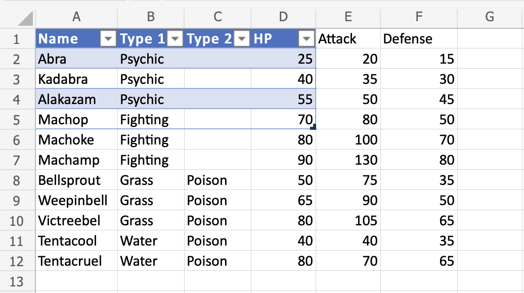
Example Sort (text)
Sort the Pokemons in the range A2:A21 by their Name, ascending from smallest to largest (A-Z).
Select A2:A21
Open the Sort & Filter menu
Click Sort Ascending
Note:A1 is not included as it is the header for the column. This is the row that is dedicated to the filter. Including it will blend it with the rest.
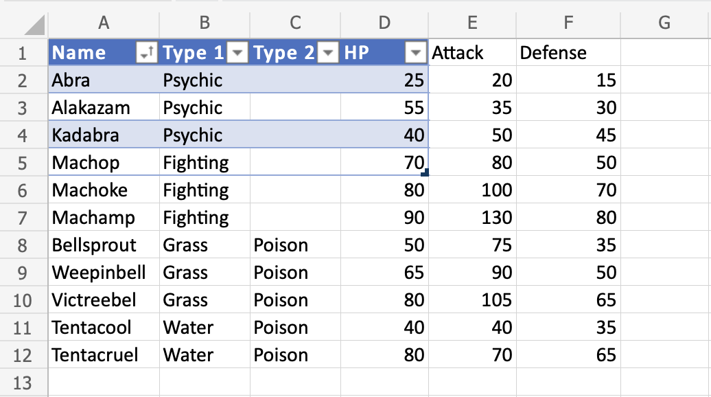
The Sort Ascending function successfully sorted the Pokemons by their Name ascending from A-Z.
Try again, this time with Sort Descending to see what that looks like!
Example Sort (numbers)
Sort the Pokemons ascending by their Total stats from smallest to largest.
Select A2:A21
Open the Sort & Filter menu
Click Sort Ascending
Great! The Pokemons were successfully sorted by their Total stats from smallest to largest. The sort commands work for both text and numbers.
A Non-Working Example (sorting one column in a range)
In this example we have two columns with related data. Column A is the Pokemons Names and Column B is their Total stats. Try sorting just one of the columns (A2:A21) ascending by their Names.
The attempt to sort results in a warning.
It is not recommended to sort the names alone because it will break the relationship between the Pokemons Names and their Total stats.
Click "Just sort" to see what happens.
This breaks the relationship with Column A and B. The Pokemons now have wrong Total stats.
Clicking the other option in the warning "Expand and Sort" makes the sort function include Column B and sorts them in relation to each other.
Sorting More Than One Column
Select the whole range when sorting ranges with more than one column.
Note: When sorting multiple columns, it will always sort by the first column (leftmost).
Select A2:B21 and sort the range ascending.
By selecting range A2:B21 it sorts correctly, keeping the relationship between the data (Column A and B).
In the next chapter you will learn about Filter.
Excel Filter
Excel Filter
Filters can be applied to sort and hide data. It makes data analysis easier.
Note: Filter is similar to formatting a table, but it can be applied and deactivated.
The menu is accessed in the default Ribbon view or in the Data section in the navigation bar.
Applying Filter
Filters are applied by selecting a range and clicking the Filter command.
It is important to have a row of headers when applying filters. Having headers is useful to make the data understandable.
Note: Filters are applied to the top row in a range.
Like in the example below, the dedicated row is row 1.
Let's apply filters to the data set, step by step.
Select range A1:E1
Click the Sort & Filter menu
Click the Filter command
New buttons have been added to the cells in the top row. This indicates that the Filter was successfully applied. The buttons can be clicked to access the different Sort & Filter options.
A Non-Working Example
Lets delete row 1 (the header row) and apply filters to the new row 1, to see what happens.
The filter is applied and has replaced the header row. It is important to dedicate a header row for the filter.
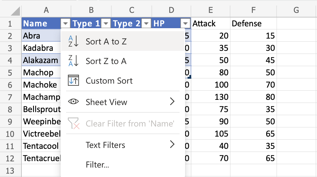
Filter options
The filter options allow for sorting and filtering.
Applying filter keeps the relationship between the columns while sorting and filtering.
Clicking the options button opens the menu.
Sorting
Ranges can be sorted and the relationship between the columns is kept.
Sort Ascending (A-Z) sorted from smallest to largest.
Sort Descending (Z-A) sorts from largest to smallest.
You can read more about Sorting in a previous .
Filtering
Filters can be applied to hide and sort data.
This is helpful for analysis, to select the data that you want to see or not.
Example Filter
Use the filter option to filter on Pokemon that is Type 1, Bug.
Step by step
Click the drop down menu on C1 () and choose the Filter option. This is the Column which holds the Type 1 data.
Note: "Items" are the different categories in that column; Grass, Fire, Water and so on.
All items are checked by default. The checked items are the ones that are shown. Uncheck to hide.
Uncheck all items, except Bug, which is the type that we want to show.
Click OK
Good job! The range was successfully sorted by Type 1, Bug. All shown Pokemons are Bug type.
Note: The unchecked rows are hidden, not deleted.
This is explained by looking at the row numbers. The numbers are jumping from 1 to 11 and 16 to 22. The rows in between are hidden.
Note: Checking the items will have the rows shown again.
Another Example
Use the filter option to filter the Pokemons which have Type 1, Bug and Type 2, Poison.
Click the filter option in D1
Uncheck all items except Poison
click OK
That is on point! We have sorted the range based on Type 1, Bug and Type 2, Poison. The filter option is helpful to make ranges easier to analyse.
Table
Ranges can be converted into tables.
Tables make it easier to structure and organize data.
Note: The filter function is similar to a table. The filter can be better used if the only function needed is to sort and filter data.
Tables connect cells in a range and put it into a fixed structure.
The cells in the table range share the same formatting.
Note: Tables can be used to prepare data for charts and pivot tables.
Tables allow for options such as:
Sort & Filter
Formatting
AutoFilling
Note: Tables can be .
Example
Formatting a range into a table will give it a new form with a fixed structure. Tables open access to new functionality such as: filtering, automations and styling.
Example (Converting a Range to Table)
How to convert range to table, step by step.
Copy the values to follow along:
Select range A1:F22
Click Insert, then Table (), in the Ribbon.
Click OK
Note: The range (A1:F22) already has headers in row 1. Unchecking the "My table has headers" option allows you to create a dedicated header if you do not already have it.
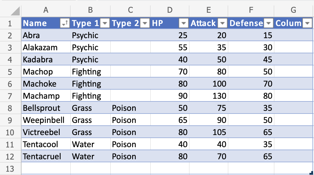
Good job! The range A1:F22 was successfully converted from range to table.
The range is now a fixed table structure and new options such as sorting and filtering are now enabled.
Applying the filter keeps the relationship between the columns while sorting and filtering.
Note: Read more about and in previous chapters.
In the next chapter you will learn about Table Design.
Table
Ranges can be converted into tables.
Tables make it easier to structure and organize data.
Note: The filter function is similar to a table. The filter can be better used if the only function needed is to sort and filter data.
Tables connect cells in a range and put it into a fixed structure.
The cells in the table range share the same formatting.
Note: Tables can be used to prepare data for charts and pivot tables.
Tables allow for options such as:
Sort & Filter
Formatting
AutoFilling
Note: Tables can be .
Example
Formatting a range into a table will give it a new form with a fixed structure. Tables open access to new functionality such as: filtering, automations and styling.
Example (Converting a Range to Table)
How to convert range to table, step by step.
Copy the values to follow along:
Select range A1:F22
Click Insert, then Table (), in the Ribbon.
Click OK
Note: The range (A1:F22) already has headers in row 1. Unchecking the "My table has headers" option allows you to create a dedicated header if you do not already have it.
Good job! The range A1:F22 was successfully converted from range to table.
The range is now a fixed table structure and new options such as sorting and filtering are now enabled.
Applying the filter keeps the relationship between the columns while sorting and filtering.
Note: Read more about and in previous chapters.
In the next chapter you will learn about Table Design.
Table Design
Tables can be customized and styled in a few clicks.
Converting a range into a table gives access to a menu called "Table Design".
The menu appears when selecting a cell in the table's range.
Excel gives tables default names such as: Table 1, Table 2, Table 3 and so on.
Note: Tables cannot be renamed in the Excel online version.
The name of the table can be found in the Table Design tab
Select the table
Click the Table design menu
See the name input field
Note: It is useful to know the table names when you have many tables in a workbook and are referring to them in formulas.
In the next chapter you will learn about resizing a table.
Table Resizing
The size of a table can be changed.
Resizing is to increase or decrease the range of the table.
There are three ways to resize a table
Resize table command
Drag to resize
Adding headers
Note: Resizing will continue formatting and formulas. This will be covered in a later chapter.
Resize Table Command
The resize table command allows you to change the size of the table by entering a range.
For example by entering A1:D10.
The command is found in the Ribbon under the Table Design tab.
Example - Resizing a Table
Convert the range into a table.
Lets resize the table from range A1:F12 to A1:F20
Select the table
Click the Table Design menu
Click the Resize Table command ()
Clicking the Resize Table command allows you to set a new range for the table.
Click the range input field
Type the new range, A1:F20
Click OK
Great! The table has been resized to from A1:F12 to A1:F20.
Drag to Resize
The table can be resized by dragging its corner.
Example - Dragging to Resize, Smaller
Change the tables size from A1:F12 to A1:D5
Press and hold the bottom right corner of the table ()
Move the pointer, marking the range A1:D5
The table range has been changed from A1:F12 to A1:D5.
Note: Cells outside of the table range are no longer included in the table. The connection between the cells created by the table is broken and they no longer have the table formatting.
Let's try to sort the Pokemon by their names to see what happens.
Click the filter option in A1
Sort by Ascending (A-Z)
The filter option only includes the Pokemon in the tables range (A1:A5). The connection to the cells outside of the table is broken.
Lets resize again, this time bigger.
Example - Dragging to Resize, Bigger
Change the tables size from A1:D5 to A1:G13
Press and hold the bottom right corner of the table ()
Move the pointer to mark A1:G13
The table range has been changed from A1:D5 to A1:G13.
The rest of the cells are now included again, and the connection between the cells is back.
Let's try to filter the Pokemon by their names to see what happens.
Click the filter option in A1
Sort by Ascending (A-Z)
Nice! The table has successfully sorted the Pokemon in the range A1:A12 by their names.
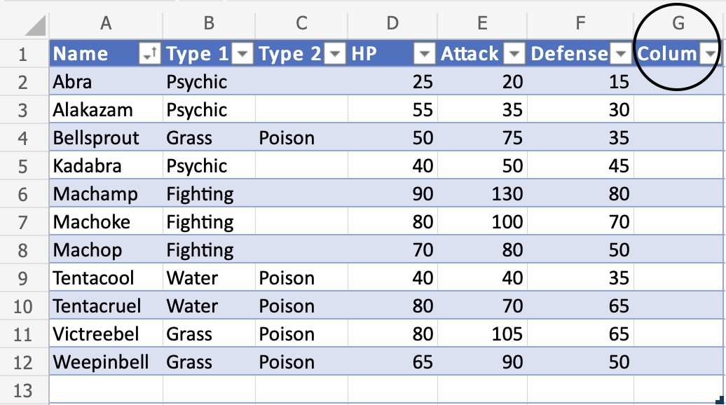
Oh wait. Something has changed. A new column (G) has appeared...
Increasing the table size will continue the formatting, formulas and add new columns.
Note: It will not overwrite the name for existing headers. It will use the value that is typed in the header cell.
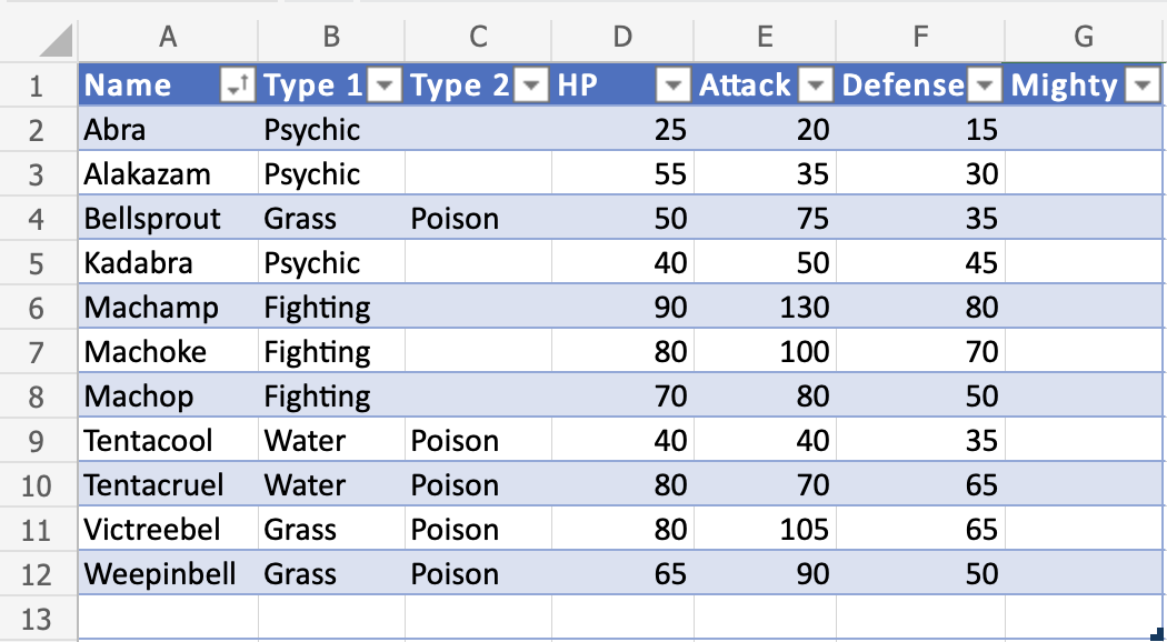
The header name can be changed.
Double click G1
Delete the text
Type "Mighty" to G1
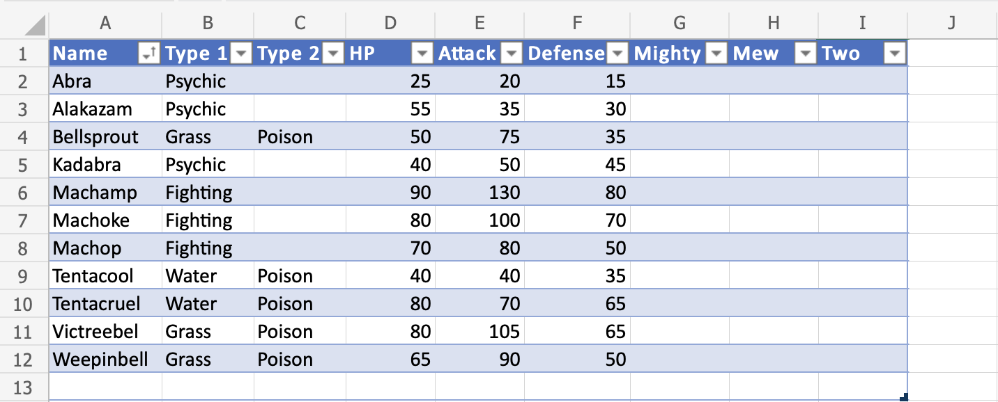
Another Example - Resize By Adding Columns
The table is automatically increased when new headers next to the table are added.
Type "Mew" to H1
Hit enter
Type "Two" to I1
Hit enter
New columns with appropriate rows are automatically added when new headers are typed.
In the next chapter you will learn about removing duplicates.
Removing Duplicates
Excel has a command to remove duplicates in tables.
Note: Duplicates are extra copies of values.
Removing duplicates are helpful when cleaning a dataset and you do not want to include copies.
The Remove Duplicate function is found in the Ribbon under the Table Design tab.
The command allows you to specify the column where you want to find and remove duplicates.
Once applied it will return the number of deleted values and how many unique ones that remains.
Note: The remove duplicate command will not ask for which duplicates to delete. Make sure that it does not delete useful data.
Examples - Remove Duplicates command
Lets try an example removing the duplicate Pokemon in the range A1:E13
Convert the range into a table.
Select the table
Click the Table Design tab ()
Click the Remove Duplicates command ()
Leave all columns checked
Click OK
Note: Unchecking a column means that it will not remove duplicates for that column.
The command returns the number of found and removed duplicates and how many unique ones that remain.
Click OK
The remove duplicates command has successfully removed the 9 duplicate Pokemon from the range and the table has been resized accordingly. The remaining 3 values are unique.
Tables can be reversed and converted back to range.
Tables can be converted to ranges by selecting a cell in the table range and clicking on the Convert to Range command.
The command to convert to range is found in the Table Design tab, in the Tools group.
Example - Convert Table to Range
Type or copy the values to follow the example.
Convert the range into a table.
Select a cell in the table range (A1:F16)
Click the Design Table tab ()
Click the Convert to Range command ()
The table is now converted into a range and it no longer has the table options available.
Note: The cell formatting is kept for the range after the conversion.
Table Style
Excel has many ready to use styles which can be applied for tables.
Table styles is to change the appearance of the table.
It can be changed to:
Make it easier to read and understand
Make it look better
The table style is Blue, Table Style Medium 2 by default.
Example: Blue, Table Style Medium 2, which is how the default looks like.
Excel has three main categories for Table styles:
Light; Light colors, more white space
Medium; Medium colors, medium white space
Dark; Dark colors, less white space
The table style can be applied in a few steps.
Example - Applying Light Style
Type or copy the values to follow along:
Convert the range into a table.
Select a cell in the table range
Click the Design Table tab ()
Click on the Table Styles option button
Note: The Table Style that is already applied has a green rectangle around it. In this case Blue, Table Style Medium 2.
Clicking the Table Style option button opens a menu with different style options.
Here the three categories are presented; Light, Medium and Dark.
Click on the Light, Green, Table Style Light 21. Found in the Light category.
Well done! The formatting of the table has changed to the light green style.
Apply Gray, Table Style Dark 4. Found in the Dark category.
Did you make it?
Note: Get familiar with the Table Styles. Try different options to see how they look.
Conditional Formatting
Conditional formatting is used to change the appearance of cells in a range based on your specified conditions.
The conditions are rules based on specified numerical values or matching text.
Changing the appearance of cells can visually highlight interesting data points for analysis.
The browser version of Excel provides a number of built-in conditions and appearances:
Note: The web browser version of Excel only offers a selection of built-in conditional formatting options.
The Excel application has the option of creating fully customized conditional formatting rules.
Conditional Formatting Example
Here, the Speed values of each pokemon is formatted with a Color Scale:
Note: Excel has several different color scales to pick from.
Color Scale Formatting Example
Highlight the Speed values of each Pokemon with Color scale conditional formatting.
Conditional formatting, step by step:
Select the range of Speed values C2:C9
Click on the Conditional Formatting icon in the ribbon, from the Home menu
Select the Color Scales from the drop-down menu
There are 12 Color Scale options with different color variations.
The color on the top of the icon will apply to the highest values.
Click on the "Green - Yellow - Red Colour Scale" icon
Now, the Speed value cells will have a colored background highlighting:
Dark green is used for the highest values, and dark red for the lowest values.
Charizard has the highest Speed value (100) and Squirtle has the lowest Speed value (43).
All the cells in the range gradually change color from green, yellow, orange, then red.
Highlight Cell Rules
Highlight Cell Rules is a premade type of conditional formatting in Excel used to change the appearance of cells in a range based on your specified conditions.
The conditions are rules based on specified numerical values, matching text, calendar dates, or duplicated and unique values.
Here is the Highlight Cell Rules part of the conditional formatting menu:
Appearance Options
The web browser version of Excel offers the following appearance options for conditionally formatted cells:
Light Red Fill with Dark Red Text
Yellow Fill with Dark Yellow Text
Green Fill with Dark Green Text
Light Red Fill
Red Text
Red Border
Here is how the options look in a spreadsheet:
Cell Rule Types
Excel offers the following cell rule types:
Highlight Cell Rule Example
The "Equal To..." Highlight Cell Rule will highlight a cell with one of the appearance options based on the cell value being equal to your specified value.
The specified value could be a particular number or particular text.
In this example, the specified value will be "48".
You can for where the Highlight Cell Rule should apply. It can be a a few cells, a single column, a single row, or a combination of multiple cells, rows and colums.
Let's apply the rule to all of the different stat values.
"Equal To..." Hightlight Cell Rule, step by step:
Select the range C2:H8 for all of the stat values
Click on the Conditional Formatting icon in the ribbon, from Home menu
Select the Highlight Cell Rules from the drop-down menu
Select the Equal To... from the menu
This will open a dialog box where you can specify the value and the appearance option.
Enter 48 into the input field
Select the appearance option "Yellow Fill with Dark Yellow Text" from the dropdown menu
Now, the cells with values equal to "48" will be highlighted in yellow:
All of Ditto's stat values are 48, so they are hightlighted.
Note: You can remove the Highlight Cell Rules with .
Highlight Cell Rules - Greater Than
Highlight Cell Rules is a premade type of conditional formatting in Excel used to change the appearance of cells in a range based on your specified conditions.
Greater Than... is one of the options for the condition.
Here is the Highlight Cell Rules part of the conditional formatting menu:
Highlight Cell Rule - Greater Than Example
The "Greater Than..." Highlight Cell Rule will highlight a cell with one of the appearance options based on the cell value being greater than to your specified value.
The specified value is typically a number, but it also works with a text value.
In this example, the specified value will be "65".
You can for where the Highlight Cell Rule should apply. It can be a a few cells, a single column, a single row, or a combination of multiple cells, rows and colums.
Let's apply the rule to the HP values.
"Greater Than..." Hightlight Cell Rule, step by step:
Select the range C2:C8 for HP values
Click on the Conditional Formatting icon in the ribbon, from Home menu
Select the Highlight Cell Rules from the drop-down menu
Select the Greater Than... from the menu
This will open a dialog box where you can specify the value and the appearance option.
Enter 65 into the input field
Select the appearance option "Green Fill with Dark Green Text" from the dropdown menu
Now, the cells with values greater than "65" will be highlighted in green:
Gyarados, Lapras and Vaporeon have HP values greater than 65, so they are hightlighted.
Note: Jolteon's HP value is 65, but is not highlighted, since the rule does not include the specified value itself.
Note: You can remove the Highlight Cell Rules with .
Highlight Cell Rule - Greater Than Example (with Text)
The "Greater Than..." Highlight Cell Rule also works with text values.
Excel will use alphabetical order (A-Z) to highlight the text values that starts with a letter that is later in the alphabet than the specified value.
In this example, the specified text value will be "Gyarados".
You can for where the Highlight Cell Rule should apply. It can be a a few cells, a single column, a single row, or a combination of multiple cells, rows and colums.
Let's apply the rule to the Name values.
"Greater Than..." Hightlight Cell Rule, step by step:
Select the range A2:A8 for Name values
Click on the Conditional Formatting icon in the ribbon, from Home menu
Select the Highlight Cell Rules from the drop-down menu
Select the Greater Than... from the menu
This will open a dialog box where you can specify the value and the appearance option.
Enter Gyarados into the input field
Select the appearance option "Yellow Fill with Dark Yellow Text" from the dropdown menu
Now, the cells with text values later in the alphabet than "Gyarados" will be highlighted in yellow:
Magikarp starts with "M", Lapras with "L", Vaporeon with "V", and Jolteon with "J".
"M", "L", "V", and "J" are all later in the alphabet than "G", which Gyarados starts with, so these all are highlighted.
But, what about the rest of the letters in the text value?
Let's see what happens if we add a fictional pokemon with a new name:
Notice that the fictional "Gzarados" is highlighted.
The Excel condition checks each letter in the specified text value from left to right.
Because the "z" in "Gzarados" comes later in the alphabet than the "y" in "Gyarados", this is considered Greater Than and is highlighted.
Highlight Cell Rules - Less Than
Highlight Cell Rules is a premade type of conditional formatting in Excel used to change the appearance of cells in a range based on your specified conditions.
Less Than... is one of the options for the condition.
Here is the Highlight Cell Rules part of the conditional formatting menu:
Highlight Cell Rule - Less Than Example
The "Less Than..." Highlight Cell Rule will highlight a cell with one of the appearance options based on the cell value being less than to your specified value.
The specified value is typically a number, but it also works with a text value.
In this example, the specified value will be "55".
You can for where the Highlight Cell Rule should apply. It can be a a few cells, a single column, a single row, or a combination of multiple cells, rows and colums.
Let's apply the rule to the Attack values.
"Less Than..." Hightlight Cell Rule, step by step:
Select the range D2:D8 for Attack values
Click on the Conditional Formatting icon in the ribbon, from Home menu
Select the Highlight Cell Rules from the drop-down menu
Select the Less Than... from the menu
This will open a dialog box where you can specify the value and the appearance option.
Enter 55 into the input field
Select the appearance option "Light Red Fill with Dark Red Text" from the dropdown menu
Now, the cells with values less than "55" will be highlighted in red:
Only Magikarp and Ditto have Attack values less than 55, so these values are highlighted.
Note: Eevees's Attack value is 55, but is not highlighted, since the rule does not include the specified value itself.
Note: You can remove the Highlight Cell Rules with .
Highlight Cell Rule - Less Than Example (with Text)
The "Less Than..." Highlight Cell Rule also works with text values.
Excel will use alphabetical order (A-Z) to highlight the text values that starts with a letter that is earlier in the alphabet than the specified value
In this example, the specified text value will be "Electric".
You can for where the Highlight Cell Rule should apply. It can be a a few cells, a single column, a single row, or a combination of multiple cells, rows and colums.
Let's apply the rule to the Type 1 values.
"Less Than..." Hightlight Cell Rule, step by step:
Select the range B2:B8 for Type 1 values
Click on the Conditional Formatting icon in the ribbon, from Home menu
Select the Highlight Cell Rules from the drop-down menu
Select the Less Than... from the menu
This will open a dialog box where you can specify the value and the appearance option.
Enter Electric into the input field
Select the appearance option "Yellow Fill with Dark Yellow Text" from the dropdown menu
Now, the cells with text values earlier in the alphabet than "Electric" will be highlighted in yellow:
Nothing seems to have changed!
Water starts with "W" and Normal starts with "N".
"W"and "N" are all later in the alphabet than "E", which Electric starts with, so none of these are highlighted.
Note: The specified value "Electric" itself is also not highlighted, because the rule only hightlights text values that are earlier in the alphabet.
So, what about the rest of the letters in the text value?
Let's see what happens if we add a fictional pokemon with a new Name and Type:
Notice that the fictional "Ficteon" has the type "Eclectic", which is highlighted.
The Excel condition checks each letter in the specified text value from left to right.
Because the "c" in "Eclectic" comes earlier in the alphabet than the "l" in "Electric", this is considered Less Than and is highlighted.
Highlight Cell Rules - Between
Highlight Cell Rules is a premade type of conditional formatting in Excel used to change the appearance of cells in a range based on your specified conditions.
Between... is one of the options for the condition.
Here is the Highlight Cell Rules part of the conditional formatting menu:
Highlight Cell Rule - Between Example
The "Between..." Highlight Cell Rule will highlight a cell with one of the appearance options based on the cell value being between two specified values.
The specified values is typically numbers, but can also be text values.
In this example, the specified values will be "79" and "100".
You can for where the Highlight Cell Rule should apply. It can be a a few cells, a single column, a single row, or a combination of multiple cells, rows and colums.
Let's apply the rule to all of the different stat values.
"Between..." Hightlight Cell Rule, step by step:
Select the range C2:H8 for all of the stat values
Click on the Conditional Formatting icon in the ribbon, from Home menu
Select the Highlight Cell Rules from the drop-down menu
Select the Between... from the menu
This will open a dialog box where you can specify the value and the appearance option.
Enter 79 and 100 into the input fields
Select the appearance option "Yellow Fill with Dark Yellow Text" from the dropdown menu
Now, the cells with values between "79" and "100" will be highlighted in yellow:
Notice that Gyarados' Defense and Special Defense, which are 79 and 100, are hightlighted.
The Between... condition includes the specified values. This is different from the and conditions, which do not include the specified values.
Note: You can remove the Highlight Cell Rules with .
Highlight Cell Rules - Equal To
Highlight Cell Rules is a premade type of conditional formatting in Excel used to change the appearance of cells in a range based on your specified conditions.
Equal To... is one of the options for the condition.
Here is the Highlight Cell Rules part of the conditional formatting menu:
Highlight Cell Rule - Equal To Example (with Numbers)
The "Equal To..." Highlight Cell Rule will highlight a cell with one of the appearance options based on the cell value being equal to your specified value.
The specified value could be a particular number or particular text.
In this example, the specified value will be "48".
You can for where the Highlight Cell Rule should apply. It can be a a few cells, a single column, a single row, or a combination of multiple cells, rows and colums.
Let's apply the rule to all of the different stat values.
"Equal To..." Hightlight Cell Rule, step by step:
Select the range C2:H8 for all of the stat values
Click on the Conditional Formatting icon in the ribbon, from Home menu
Select the Highlight Cell Rules from the drop-down menu
Select the Equal To... from the menu
This will open a dialog box where you can specify the value and the appearance option.
Enter 48 into the input field
Select the appearance option "Yellow Fill with Dark Yellow Text" from the dropdown menu
Now, the cells with values equal to "48" will be highlighted in yellow:
All of Ditto's stat values are 48, so they are hightlighted.
Note: You can remove the Highlight Cell Rules with .
Highlight Cell Rule - Equal To Example (with Text)
The "Equal To..." Highlight Cell Rule also works with text values.
In this example, the specified text value will be "Magikarp".
You can for where the Highlight Cell Rule should apply. It can be a a few cells, a single column, a single row, or a combination of multiple cells, rows and colums.
Let's apply the rule to the Name values.
"Equal To..." Hightlight Cell Rule, step by step:
Select the range A2:A8 for Name values
Click on the Conditional Formatting icon in the ribbon, from Home menu
Select the Highlight Cell Rules from the drop-down menu
Select the Equal To... from the menu
This will open a dialog box where you can specify the value and the appearance option.
Enter Magikarp into the input field
Select the appearance option "Yellow Fill with Dark Yellow Text" from the dropdown menu
Now, the cells with text values equal to "Magikarp" will be highlighted in yellow:
Note: The Equal To... Highlight Cell Rule will highlight cells that exactly matches the specified value.
You can use the rule for highlighting cells that have values with any part matching the specified value.
Highlight Cell Rules - Text That Contains
Highlight Cell Rules is a premade type of conditional formatting in Excel used to change the appearance of cells in a range based on your specified conditions.
Text That Contains... is one of the options for the condition.
Here is the Highlight Cell Rules part of the conditional formatting menu:
Highlight Cell Rule - Text That Contains Example (with Text)
The "Text That Contains..." Highlight Cell Rule will highlight a cell with one of the appearance options based on a part of the cell value containing your specified value.
The specified value is typically text, but also works with a numerical value.
In this example, the specified value will be "Pidge".
You can for where the Highlight Cell Rule should apply. It can be a a few cells, a single column, a single row, or a combination of multiple cells, rows and colums.
Let's apply the rule to the Name values.
"Text That Contains..." Hightlight Cell Rule, step by step:
Select the range A2:A8 for the Name values
Click on the Conditional Formatting icon in the ribbon, from Home menu
Select the Highlight Cell Rules from the drop-down menu
Select the Text That Contains... from the menu
This will open a dialog box where you can specify the value and the appearance option.
Enter Pidge into the input field
Select the appearance option "Yellow Fill with Dark Yellow Text" from the dropdown menu
Now, the cells with values Text That Contains "Pidge" will be highlighted in yellow:
The names "Pidgey", "Pidgeot", and "Pidgeotto" all start with "Pidge", so all these cells are highlighted.
Note: The Text That Contains rule works with any part of the cell values.
Like in the example below:
Highlight Cell Rule - Text That Contains Example 2 (with Text)
The "Text That Contains..." Highlight Cell Rule will highlight a cell with one of the appearance options based on a part of the cell value containing your specified value.
The specified value is typically text, but also works with a numerical value.
In this example, the specified value will be "row".
You can for where the Highlight Cell Rule should apply. It can be a a few cells, a single column, a single row, or a combination of multiple cells, rows and colums.
Let's apply the rule to the Name values.
"Text That Contains..." Hightlight Cell Rule, step by step:
Select the range A2:A8 for the Name values
Click on the Conditional Formatting icon in the ribbon, from Home menu
Select the Highlight Cell Rules from the drop-down menu
Select the Text That Contains... from the menu
This will open a dialog box where you can specify the value and the appearance option.
Enter row into the input field
Select the appearance option "Yellow Fill with Dark Yellow Text" from the dropdown menu
Now, the cells with values Text That Contains "row" will be highlighted in yellow:
The names "Spearow" and "Fearow" both end with "row", so both cells are highlighted.
Note: You can remove the Highlight Cell Rules with .
Highlight Cell Rule - Text That Contains Example (with Numbers)
The "Text That Contains..." Highlight Cell Rule also works with numbers.
In this example, the specified text value will be "7".
You can for where the Highlight Cell Rule should apply. It can be a a few cells, a single column, a single row, or a combination of multiple cells, rows and colums.
Let's apply the rule to all the different stat values.
"Text That Contains..." Hightlight Cell Rule, step by step:
Select the range C2:H8 for all the stat values
Click on the Conditional Formatting icon in the ribbon, from Home menu
Select the Highlight Cell Rules from the drop-down menu
Select the Text That Contains... from the menu
This will open a dialog box where you can specify the value and the appearance option.
Enter 7 into the input field
Select the appearance option "Green Fill with Dark Green Text" from the dropdown menu
Now, the cells with values That Contains "7" anywhere will be highlighted in green:
Note: The Text That Contains... Highlight Cell Rule will highlight cells that have values with any part matching the specified value.
You can use the rule for highlighting cells that exactly matches the specified value.
Highlight Cell Rules - A Date Occurring
Highlight Cell Rules is a premade type of conditional formatting in Excel used to change the appearance of cells in a range based on your specified conditions.
A Date Occurring... is one of the options for the condition.
Here is the Highlight Cell Rules part of the conditional formatting menu:
Highlight Cell Rule - A Date Occurring Example
The "A Date Occurring..." Highlight Cell Rule will highlight a cell with one of the appearance options based on the cell value relative to a specified time frame.
The time frame can be:
Yesterday
Today
Tomorrow
In the last 7 days
Last Week
This Week
Next Week
Last Month
This Month
Next Month
In this example, the specified time frame will be "next month".
You can for where the Highlight Cell Rule should apply. It can be a a few cells, a single column, a single row, or a combination of multiple cells, rows and colums.
Let's apply the rule to the Birthday values.
"A Date Occurring..." Hightlight Cell Rule, step by step:
Select the range C2:C19 for the Birthday values
Click on the Conditional Formatting icon in the ribbon, from Home menu
Select the Highlight Cell Rules from the drop-down menu
Select the A Date Occurring... from the menu
This will open a dialog box where you can specify the value and the appearance option.
Select "Next Month" from the dropdown menu
Select the appearance option "Yellow Fill with Dark Yellow Text" from the dropdown menu
Now, the cells with values A Date Occurring next month will be highlighted in yellow:
Note: In this example, the next month happens to be September.
Turtwig, Chimchar, Piplup, Snivy, Tepig, and Oshawott all have birthdays in September, so their cells are hightlighted.
Note: You can remove the Highlight Cell Rules with .
Highlight Cell Rules - Duplicate and Unique Values
Highlight Cell Rules is a premade type of conditional formatting in Excel used to change the appearance of cells in a range based on your specified conditions.
Duplicate Values.. is one of the options for the condition, and can check for both duplicate and unique values.
Here is the Highlight Cell Rules part of the conditional formatting menu:
Highlight Cell Rule - Duplicate Value Example
The "Duplicate Value..." Highlight Cell Rule will highlight a cell with one of the appearance options based on the cell value being the same as other cells in the range.
You can for where the Highlight Cell Rule should apply. It can be a a few cells, a single column, a single row, or a combination of multiple cells, rows and columns.
Let's apply the rule to all of the cells values.
"Equal To..." Hightlight Cell Rule, step by step:
Select the range A2:H8
Click on the Conditional Formatting icon in the ribbon, from Home menu
Select the Highlight Cell Rules from the drop-down menu
Select the Duplicate Values... from the menu
This will open a dialog box where you can specify the value and the appearance option.
Select Duplicate
Select the appearance option "Yellow Fill with Dark Yellow Text" from the dropdown menu
Now, all the cells in the range that have the same value as another cell are hightlighted in yellow:
All of Ditto's stat values are 48 and all of Mew's stat values are 100, so they are all hightlighted.
All of the Dittos and all of the Normal Type values are also highlighted.
Note: You can remove the Highlight Cell Rules with .
Highlight Cell Rule - Unique Value Example
The "Duplicate Values..." Highlight Cell Rule can also find and highlight Unique Values.
Let's apply this to the same set of data:
You can for where the Highlight Cell Rule should apply. It can be a a few cells, a single column, a single row, or a combination of multiple cells, rows and columns.
Let's apply the rule to all of the cells values.
"Equal To..." Hightlight Cell Rule, step by step:
Select the range A2:H8
Click on the Conditional Formatting icon in the ribbon, from Home menu
Select the Highlight Cell Rules from the drop-down menu
Select the Duplicate Value... from the menu
This will open a dialog box where you can specify the value and the appearance option.
Select Unique from the dropdown menu
Select the appearance option "Green Fill with Dark Green Text" from the dropdown menu
Now, the cells with unique values will be highlighted in green:
Mew and Psychic only appears once in the range, so these values are highlighted.
Note: You can remove the unwanted duplicates from a table with .
Top/Bottom Rules
Top/Bottom Rules are premade types of conditional formatting in Excel used to change the appearance of cells in a range based on your specified conditions.
Here is the Top/Bottom Rules part of the conditional formatting menu:
Appearance Options
The web browser version of Excel offers the following appearance options for conditionally formatted cells:
Light Red Fill with Dark Red Text
Yellow Fill with Dark Yellow Text
Green Fill with Dark Green Text
Light Red Fill
Red Text
Red Border
Here is how the options look in a spreadsheet:
Top/Bottom 10 Items Example
The "Top 10 Items..." and "Bottom 10 Items..." rules will highlight cells with one of the appearance options based on the cell value being the top or bottom values in a range.
Note: The default number of items is 10, but you can specify any whole number up to 1000 for Top/Bottom Items to be highlighted.
You can for where the Highlight Cell Rule should apply. It can be a a few cells, a single column, a single row, or a combination of multiple cells, rows and colums.
Let's first apply the Top 10 Items... rule to the Speed values.
"Top 10 Items..." Rule, step by step:
Select the range C2:C31 for Speed values
Click on the Conditional Formatting icon in the ribbon, from Home menu
Select the Top/Bottom Rules from the drop-down menu
Select the Top 10 Items... from the menu
This will open a dialog box where you can specify the value and the appearance option.
Leave the default value 10 in the input field
Select the appearance option "Green Fill with Dark Green Text" from the dropdown menu
Now, the 10 cells with the top values will be highlighted in green:
Great! Now, the top 10 Speed values are easily identified.
Let's try the same with the bottom 10 Speed values.
Note: Multiple rules can be applied to the same range.
Repeat the steps, but instead choose Bottom 10 Items... in the menu and select the "Light Red Fill with Dark Red Text" appearance option.
Now, the slowest values are also highlighted:
Notice that there are actually 11 items highlighted in red. Why could this be?
Let's with descending Speed values for a clue:
We can see that both Pidgey and Nidorina have a Speed of 56. So, they are tied for the 10th bottom value.
Note: When using the Top/Bottom 10... conditional formatting, values that tie will all be highlighted.
Top/Bottom 10% Example
The "Top 10%..." and "Bottom 10%..." rules will highlight cells with one of the appearance options based on the cell value being the top or bottom percent of values in a range.
Note: The default percent of items is 10, but you can specify any whole number up to 100 for Top/Bottom Percent to be highlighted.
Let's apply Top and Bottom 10% rules to the same dataset with sorted Speed values:
You can for where the Highlight Cell Rule should apply. It can be a a few cells, a single column, a single row, or a combination of multiple cells, rows and colums.
Let's first apply the Bottom 10%... rule to the Speed values.
"Bottom 10%..." Rule, step by step:
Select the range C2:C31 for Speed values
Click on the Conditional Formatting icon in the ribbon, from Home menu
Select the Top/Bottom Rules from the drop-down menu
Select the Bottom 10%... from the menu
This will open a dialog box where you can specify the value and the appearance option.
Leave the default value 10 in the input field
Select the appearance option "Light Red Fill with Dark Red Text" from the dropdown menu
Now, the bottom 10% of cells will be highlighted in red:
Notice that there are 3 highlighted cells.
There are 30 cells in the range, so 10% of that is 3 cells.
Note: The number of cells will be rounded down to the closest whole number based on the percent.
For example:
6% of 30 is 1.8, which will be rounded down to 1 cell
7% of 30 is 2.1, which will be rounded down to 2 cells
Let's try the same with the top 10% Speed values.
Repeat the steps, but instead choose Top 10%... in the menu and select the "Green Fill with Dark Green Text" appearance option.
Now, the fastest values are also highlighted:
Notice that there are actually 4 items highlighted in green.
We can see that both Charizard and Fearow have a Speed of 100. So, they are tied for the 3rd top value.
Both are included in the top 10% and are highlighted.
Note: You can remove the Highlight Cell Rules with .
Above and Below Average Rules
Above and Below Average Rules are premade types of conditional formatting in Excel used to change the appearance of cells in a range based on your specified conditions.
Above and Below Average Rules are found in the Top/Bottom Rules part of the conditional formatting menu:
Appearance Options
The web browser version of Excel offers the following appearance options for conditionally formatted cells:
Light Red Fill with Dark Red Text
Yellow Fill with Dark Yellow Text
Green Fill with Dark Green Text
Light Red Fill
Red Text
Red Border
Here is how the options look in a spreadsheet:
Above and Below Average Example
The "Above Average" rule will highlight cells with one of the appearance options based on the cell value being the above the average value in a range.
Note: You can use Excel to calcluate the of a range, like in the example data below:
Note: The Average value row is separated from the data with a visual border. Check out how to add this in the .
You can for where the Highlight Cell Rule should apply. It can be a a few cells, a single column, a single row, or a combination of multiple cells, rows and colums.
Let's first apply the Above Average rule to the HP values.
"Above Average" Rule, step by step:
Select the range C2:C11 for HP values
Click on the Conditional Formatting icon in the ribbon, from Home menu
Select the Top/Bottom Rules from the drop-down menu
Select Above Average from the menu
This will open a dialog box where you can specify the value and the appearance option.
Select the appearance option "Green Fill with Dark Green Text" from the dropdown menu
Now, the cells with above average HP values (more than 77.2) will be highlighted in green:
Let's try the same with the below average HP values.
Note: Multiple rules can be applied to the same range.
Repeat the steps, but instead choose Below Average in the menu and select the "Light Red Fill with Dark Red Text" appearance option.
Now, the below average values are also highlighted:
Note: You can remove the Highlight Cell Rules with .
Notice that there are more below average values than above average values. Why could this be?
The number of above or below average value cells in a range will depend on the actual values in the range.
If some values in the range are extra large this will increase the average by a lot.
Let's add a fictional Pokemon with a very high HP stat value to illustrate this:
The fictional Wigglytuffest has 1000 HP, which increases the average value all the way up to more than 161.
Now, only Wigglytuffest has an above average HP stat value, and every other Pokemon has below average HP stat values.
Note: This kind of average value is referred to as the mean.
You can learn more about different kinds of average values are calculated in the .
Data Bars
Data Bars are premade types of conditional formatting in Excel used to add colored bars to cells in a range to indicate how large the cell values are compared to the other values.
Here is the Data Bars part of the conditional formatting menu:
Data Bars Example
You can for where the Highlight Cell Rule should apply. It can be a a few cells, a single column, a single row, or a combination of multiple cells, rows and colums.
Note: The size of the data bars depends on the smallest and largest cell value in the range.
Let's apply the Data Bars conditional formatting to the Speed values.
"Data Bars", step by step:
Select the range C2:C10 for Speed values
Click on the Conditional Formatting icon in the ribbon, from Home menu
Select Data Bars from the drop-down menu
Select the "Green Data Bars" color option from the Gradient Fill menu
Note: Both Gradient Fill and Solid Fill work the same way. The only difference between those, and the color options are aesthetic.
Now, all of the Speed value cells have a green bar showing how big the value is compared to the other values in the range:
Electrode has the highest value, 140, so the bar fills the entire cell.
The other bars are scaled relative to the highest value and 0 by default.
Exeggcute has the lowest value, 40, so this is the shortest bar. Though, it is larger than 0, so there is still a small bar.
Let's see what happens if we add a fictional Pokemon with a 0 Speed value:
The fictional Neutrinode has a Speed value of 0, so this becomes an invisible "minimum" bar.
Let's see what happens if we add another fictional Pokemon with a negative Speed value:
Now, the fictional Positrode has the lowest Speed value, -140, so this becomes an invisible "minimum" bar.
Notice that all the other bars have now been scaled relative to the new minimum (-140).
Neutrinode's Speed value of 0 is now in the middle between -140 and 140, so the cell has a bar filling half the cell.
Electrode still has the highest Speed value, 140, so this bar still fills the entire cell.
Note: You can remove the Highlight Cell Rules with .
Color Scales
Color Scales are premade types of conditional formatting in Excel used to highlight cells in a range to indicate how large the cell values are compared to the other values in the range.
Here is the Color Scales part of the conditional formatting menu:
Color Scale Formatting Example
Highlight the Speed values of each Pokemon with Color Scale conditional formatting.
Color Scales, step by step:
Select the range of Speed values C2:C8
Click on the Conditional Formatting icon in the ribbon, from the Home menu
Select the Color Scales from the drop-down menu
There are 12 Color Scale options with different color variations.
The color on the top of the icon will apply to the highest values.
Click on the "Green - Yellow - Red Colour Scale" icon
Now, the Speed value cells will have a colored background highlighting:
Dark green is used for the highest values, and dark red for the lowest values.
Rapidash has the highest Speed value (105) and Slowpoke has the lowest Speed value (15).
All the cells in the range gradually change color from green, yellow, orange, then red.
Note: The color formatting is relative to the smallest and largest cell values in the range.
Let's see what happens if we add a fictional Pokemon with an even slower Speed value than Slowpoke:
Now, the fictional Slowestpoke has the lowest Speed value of 1, which is highlighted in dark red.
Notice that the color of Slowpoke's Speed value now is highlighted in orange instead of dark red.
Let's see what happens if we add another fictional Pokemon that is faster than any of the other Pokemon:
The fictional Fastestpoke has a higher Speed value (200) than any of the other pokemon and is highlighted in dark green.
Rapidash' Speed value of 105 is no longer the highest value and is highlighted with a lighter green.
Notice that the Speed values of the other Pokemon also change as the highest value in the range is now 200 instead of 105.
Note: You can remove the Highlight Cell Rules with .
Icon Sets
Icon Sets are premade types of conditional formatting in Excel used to add icons to cells in a range to indicate how large the cell values are compared to the other values in the range.
Note: Icon Sets can be used together with other conditional formatting rules.
Icon Sets Options
Excel has a number of different icon sets, organized as:
Directional
Shapes
Indicators
Ratings
Icon Set Formatting Example
Add icons to the Speed values of each Pokemon with Icon Set conditional formatting.
Icon Sets, step by step:
Select the range of Speed values C2:C10
Click on the Conditional Formatting icon in the ribbon, from the Home menu
Select the Icon Sets from the drop-down menu
Click on the "3 Traffic Lights (Unrimmed)" option
Now, the Speed value cells will have icons indicating how large the values are compared to the other values in the range:
The green traffic light is used for the highest values, yellow for the middle values, and red for the lowest values.
Excel automatically calculates and chooses which values get which colored traffic light icon.
Note: You can remove the Highlight Cell Rules with .
Excel Manage Rules
Conditional Formatting rules can be managed and removed using the Clear Rules and Manage Rules features.
Here is the Clear Rules part of the conditional formatting menu:
You can remove all the rules from a selected range of cells or from the entire spreadsheet using the Clear Rules menu options.
Conditional Formatting - Manage Rules Example
You can also use the Manage Rules menu option to clear conditional formatting rules.
Let's remove the Color Scale rule applied to all the Stat values:
Select the range C2:H9.
Select the Manage Rules option from the Conditional Formatting menu in the Home menu.
This box will appear on the right-hand side of your spreadsheet:
This will show all the active rules that are applied to the selected range.
It will also indicate which cells the rule is applied to. Which, in this example, is C2:H9.
Note: In the web browswer version of Excel, the only thing that can be managed is removing the rules.
Clicking on the recycling bin icon will remove a particular rule.
Now, the cells no longer have conditional formatting.
Excel Charts
Charts are visual representations of data used to make it more understandable.
Commonly used charts are:
Pie chart
Column chart
Line chart
Different charts are used for different types of data.
Note: Charts are also called graphs and visualizations.
The chart above is a column chart representing the number of Pokemons in each generation.
Note: In some cases the data has to be processed before plotted into a chart.
Charts can easily be created in a few steps in Excel.
Creating a Chart in Excel
Creating a chart, step by step:
Select the range A1:A8
Click on the Insert menu, then click on the Line menu () and choose Line () from the drop-down menu
Note: This menu is accessed by .
You should now get this chart:
Excellent! You have now created your first chart.
Note: The cells 9 and 10 were not selected in the range, and therefore not included in the graph.
Creating Another Chart in Excel
Lets compare the stats for the Pokemons; Charmander, Squirtle and Bulbasaur using a column chart.
Select the range A1:G4
Click on the insert menu, then click on the column menu () and choose Clustered Column () from the drop-down menu
Note: This menu is accessed by .
You should now get this chart:
The chart gives a visual overview for the Pokemons stats.
Charmander, represented by the orange bars, and has the highest speed. Squirtle, represented by the gray bars, has the highest defense.
Note: The default chart title is "Chart Title". It can be changed. You will learn about in a later chapter.
Bar Charts
Bar charts show the data as vertical bars.
The chart above represents the number of Pokemons in each generation.
Similar to column charts, bar charts are suited for representing values of qualitative (categorical) data.
Note: You can read more qualitative (categorical) data at .
There are three different type of bar charts:
Clustered bar()
Stacked bar()
100% stacked bar()
Clustered Bar Chart
Clustered Bar charts are used when the value of data is important but the order is not.
Example With One Data Column
We want to find the number of generation 1 Pokemons with types "Grass", "Fire", "Water" and "Bug".
You can copy the values to follow along:
Select the range A1:B5
Click on the insert menu, then click on the bar menu () and choose Clustered Bar () from the drop-down menu
Note: This menu is accessed by .
Well Done! Following the steps above will give you the chart below.
The chart gives a visual overview for the "Grass", "Fire", "Water" and "Bug" type Pokemons in generation 1.
Type "Water" has the most Pokemons in the first generation.
Example With Two Data Columns
Now let's do the same for generation 2 Pokemons and compare the results with the last example.
Select the range A1:C5
Click on the insert menu, then click on the bar menu () and choose Clustered Bar () from the drop-down menu
Note: This menu is accessed by .
You should get the chart below:
The chart gives a visual overview for the "Grass", "Fire", "Water" and "Bug" type Pokemons in generation 1 and 2.
Generation 1 is shown in blue and generation 2 is shown in orange.
Type "Water" has the most Pokemons in both generations
Also, all the types in generation 2 have less members than generation 1.
Stacked Bar Chart
Stacked bar charts are used to highlights the total amount of contribution for each category.
This is done by stacking the bars at the end of each other.
The charts are used when you have more than one data column.
Example
We want to find out the total number of generation 1 and 2 Pokemons in each of these type 1 categories: "Grass", "Fire", "Water" and "Bug".
You can copy the values to follow along:
Select the range A1:C5
Click on the insert menu, then click on the bar menu () and choose Stacked Bar () from the drop-down menu
Note: This menu is accessed by .
Following the steps above, you will get the following chart:
The chart gives a visual overview for the total number of "Grass", "Fire", "Water" and "Bug" type Pokemons in both generation 1 and 2.
Generation 1 Pokemons are shown in blue and generation 2 Pokemons are shown in orange.
This chart shows that "Water" type Pokemons are the most common and "Fire" type Pokemons are the least common.
100% Stacked Bar Chart
100% Stacked Bar is used to highlights the proportion of contribution for each data column in a category.
This is done by scaling the total value of each category in a stacked bar chart to 100.
The charts are used when you have more than one data column.
Example
We want to find out the proportion of Pokemon types "Grass", "Fire", "Water" and "Bug" in generation 1 and 2.
You can copy the values to follow along:
Select the range A1:C5
Click on the insert menu, then click on the bar menu () and choose 100% Stacked Bar () from the drop-down menu
Note: This menu is accessed by .
Following the steps above, you will get the following chart:
The chart gives a visual overview for the proportion of "Grass", "Fire", "Water" and "Bug" type Pokemons in both generation 1 and 2.
Generation 1 Pokemons are shown in blue and generation 2 Pokemons are shown in orange.
This chart shows that more than half of Pokemons are in generation 1.
Column Charts
Column charts show the data as vertical bars.
Column charts are suited for representing values of qualitative (categorical) data.
Note: You can read more qualitative (categorical) data at .
Excel has three different types of column charts:
Clustered column()
Stacked column()
100% Stacked column()
Clustered Column Chart
Clustered Column charts are used when the value of data is important but the order is not.
Example With One Data Column
We want to find the number of generation 1 Pokemons with types "Grass", "Fire", "Water" and "Bug".
You can copy the values to follow along:
Select the range A1:B5
Click on the insert menu, then click on the column menu () and choose Clustered Column () from the drop-down menu
Note: This menu is accessed by .
Nicely Done! Following the steps above will give you the chart below.
The chart gives a visual overview for the "Grass", "Fire", "Water" and "Bug" type Pokemons in generation 1.
Type "Water" has the most Pokemons in the first generation.
Example With Two Data Columns
Now let's do the same for generation 2 Pokemons and compare the results with the last example.
Select the range A1:C5
Click on the insert menu, then click on the column menu () and choose Clustered Column () from the drop-down menu
Note: This menu is accessed by .
You should get the chart below:
The chart gives a visual overview for the "Grass", "Fire", "Water" and "Bug" type Pokemons in generation 1 and 2.
Generation 1 is shown in blue and generation 2 is shown in orange.
Type "Water" has the most Pokemons in both generations
Also, there are more Pokemons in generation 1 than 2.
Stacked Column Chart
Stacked Column charts are used to highlights the total amount of contribution for each category.
This is done by stacking columns on top of each other.
The charts are used when you have more than one data column.
Example
We want to find out the total number of generation 1 and 2 Pokemons in each of these type 1 categories: "Grass", "Fire", "Water" and "Bug".
You can copy the values to follow along:
Select the range A1:C5
Click on the insert menu, then click on the column menu () and choose Clustered Column () from the drop-down menu
Note: This menu is accessed by .
Following the steps above, you will get the following chart:
The chart gives a visual overview for the total number of "Grass", "Fire", "Water" and "Bug" type Pokemons in both generation 1 and 2.
Generation 1 Pokemons are shown in blue and generation 2 Pokemons are shown in orange.
This chart shows that "Water" type Pokemons are the most common and "Fire" type Pokemons are the least common.
100% Stacked Column Chart
100% Stacked Column is used to highlights the proportion of contribution for each data column in a category.
This is done by scaling the total value of each category in a stacked column chart to 100.
The charts are used when you have more than one data column.
Example
We want to find out the proportion of Pokemon types "Grass", "Fire", "Water" and "Bug" in generation 1 and 2.
You can copy the values to follow along:
Select the range A1:C5
Click on the insert menu, then click on the column menu () and choose Clustered Column () from the drop-down menu
Note: This menu is accessed by .
Following the steps above, you will get the following chart:
The chart gives a visual overview for the proportion of "Grass", "Fire", "Water" and "Bug" type Pokemons in both generation 1 and 2.
Generation 1 Pokemons are shown in blue and generation 2 Pokemons are shown in orange.
This chart shows that more than half of Pokemons are in generation 1.
Pie Charts
Pie charts arrange the data as slices in a circle.
Pie charts are used for representing values of qualitative (categorical) data.
Pie charts show the contribution of each category to the total.
Note: You can read more about qualitative (categorical) data at .
Excel has two types of pie charts:
2-D pie ()
Doughnut ()
2-D Pie Chart
Pie charts arrange the data as slices in a circle.
2-D pie charts are used when you only have one data column.
Example
Showing the proportion of 1st generation Grass, Fire, Water, and Bug type Pokemon.
You can copy the values to follow along:
Select the range A1:B5
Click on the Insert menu, then click on the Pie menu () and choose Pie () from the drop-down menu
Note: This menu is accessed by .
You should get the chart below:
The chart gives a visual overview of the number of 1st generation Grass, Fire, Water and Bug type Pokemon.
Type "Grass" is shown in blue, "Fire" in orange, "Water" in gray and "Bug" in yellow.
Type "Water" has the most Pokemon in the first generation.
Note: The chart can be customized by adding labels. This can make it easier to understand the differences between categories.
Doughnut Chart
Doughnut charts arrange the data as slices in a circle with hollow center.
Doughnut charts are often used when you have more than one data column.
Note: A doughnut chart with one data column shows the same information as a 2-D pie chart.
Example
We want to find the proportion of types "Grass", "Fire", "Water" and "Bug". in generation 1 Pokemon and compare it to the proportions in generation 2.
You can copy the values to follow along:
Select the range A1:C5
Click on the Insert menu, then click on the Pie menu () and choose Doughnut () from the drop-down menu
Note: This menu is accessed by .
Following the steps above, you will get the following chart:
The chart gives a visual overview of the number of 1st and 2nd generation Grass, Fire, Water and Bug type Pokemon.
Generation 1 Pokemon are shown in the inner circle and generation 2 Pokemon are shown in the outer circle.
Type "Grass" is shown in blue, "Fire" in orange, "Water" in gray and "Bug" in yellow.
This chart shows that "Water" type Pokemon are the most common in both generations.
Note: The chart can be customized by adding labels. This can make it easier to understand the differences between different categories.
Note: Based on this chart, you cannot say which generation has more Pokemon.
Line Charts
Line charts show the data as a continuous line.
Line charts are typically used for showing trends over time.
In Line charts, the horizontal axis typically represents time.
Line charts are used with data which can be placed in an order, from low to high.
Note: Data which can be placed in an order, from low to high, like numbers and letter grades from A to F are called ordinal data. You can read more about ordinal data at
Excel has six types of line charts:
Line ()
Line with Markers ()
Stacked Line ()
Stacked Line with Markers ()
100% Stacked Line ()
100% Stacked Line with Markers ()
Line
Line charts are used for showing data ordered from low to high.
Example
Let's see the stats change for Bulbasaur evolutions.
Copy the values to follow along:
Select the range A1:C4 for labels and data
Note: This menu is accessed by .
Click on the Insert menu, then click on the Line menu () and choose Line () from the drop-down menu
You should get the chart below:
The chart gives a visual overview for the Pokemon stats.
Bulbasaur evolutions are shown on the horizontal axis.
HP stat is shown in blue and Attack stat is shown in orange.
The chart shows that with each evolution, the stats increase.
Fantastic! Now let's plot more stats on the chart.
Select the range A1:D4 for labels and data
Click on the Insert menu, then click on Line menu () and choose Line () from the drop-down menu
You should get the chart below:
Wait a minute. Something doesn't seem right.
Suddenly, Bulbasaur's evolutions are not shown on the horizontal axis. Instead, it is the stats.
What's happening?
Note: Excel checks the number of rows and columns included in the chart and automatically places the larger number on the horizontal axis.
Luckily, there is a simple fix.
Click on the the chart, then chick on the Chart tab and finally Click on Switch Row/Column.
The outcome is this chart which has Bulbasaur evolutions on the horizontal axis.
Line with Markers
Line with markers highlights data points with markers on a line chart.
Example
Let's chart the average HP, Attack and Defense over all the Pokemon generations.
Copy the values to follow along:
Note: This data is rounded to one decimal.
Select the range A1:D7 for labels and data
Note: This menu is accessed by .
Click on the Insert menu, then click on the Line menu () and choose Line with Markers () from the drop-down menu
You should get the chart below:
The chart gives a visual overview for average Pokemon stats over generations.
Average HP is shown in blue, average attack is shown in orange and average defense is shown in gray.
The horizontal axis shows the generations.
This chart shows that the average of all stats in the 2nd generation is very close to each other and 5th generation Pokemon have on average the highest attack.
Stacked Line
Stacked Line charts show the contribution to trends in the data.
This is done by stacking lines on top of each other.
Stacked Line charts are used with data which can be placed in an order, from low to high.
The charts are used when you have more than one data column which all add up to the total trend.
Note: Data which can be placed in an order, from low to high, like numbers and letter grades from A to F are called ordinal data. You can read more about ordinal data at
Example
Let's see how the average stats add up across Pokemon generations
Copy the values to follow along:
Note: This data is rounded to one decimal.
Select the range A1:D7 for labels and data
Note: This menu is accessed by .
Click on the Insert menu, then click on the Line menu () and choose Stacked Line () from the drop-down menu
You should get the chart below:
The chart gives a visual overview for the average Pokemon stats over generations.
The blue line shows the average HP, the orange line show the addition of average HP and Average attack. Finally, the gray line shows the sum of all the stats once all the average stats are added.
This chart shows that 4th generation Pokemon have the highest stats on average.
Stacked Line with Markers
Stacked line with markers highlights data points with markers on a stacked line chart.
Example
Let's see how the average stats add up across Pokemon generations
Copy the values to follow along:
Note: This data is rounded to one decimal.
Select the range A1:D7 for labels and data
Note: This menu is accessed by .
Click on the Insert menu, then click on the Line menu () and choose Stacked Line with Markers () from the drop-down menu
You should get the chart below:
The chart gives a visual overview for the average Pokemon stats over generations.
The blue line shows the average HP, the orange line show the addition of average HP and Average attack. Finally, the gray line shows the sum of all the stats once all the average stats are added.
This chart shows that 4th generation Pokemon have the highest stats on average.
100% Stacked Line
100% Stacked Line charts show the proportion of contribution to trends in the data.
This is done by scaling the lines so that the total is 100%.
100% Stacked Line charts are used with data which can be placed in an order, from low to high.
The charts are used when you have more than one data column which all add up to the total trend.
Note: Data which can be placed in an order, from low to high, like numbers and letter grades from A to F are called ordinal data. You can read more about ordinal data at
Example
Let's see how the average stats add up across Pokemon generations
Copy the values to follow along:
Note: This data is rounded to one decimal.
Select the range A1:D7 for labels and data
Note: This menu is accessed by .
Click on the Insert menu, then click on the Line menu () and choose 100% Stacked Line () from the drop-down menu
You should get the chart below:
The chart gives a visual overview for the average Pokemon stats over generations.
The blue line shows how much the average HP contribute to the overall. The orange line shows how much the average Attack contribute to the total and finally, the gray line shows all the sum of all the stats scaled to 100%.
This chart shows that in the second generation, HP contributes more to the overall compared to other generations.
100% Stacked Line with Markers
100% stacked line with markers highlights data points with markers on a 100% stacked line chart.
Example
Let's see how the average stats add up across Pokemon generations
Copy the values to follow along:
Note: This data is rounded to one decimal.
Select the range A1:D7 for labels and data
Note: This menu is accessed by .
Click on the Insert menu, then click on the Line menu () and choose 100% Stacked Line with Markers () from the drop-down menu
You should get the chart below:
The chart gives a visual overview for the average Pokemon stats over generations.
The blue line shows how much the average HP contribute to the overall. The line orange line shows how much the average Attack contribute to the total and finally, the gray line shows all the sum of all the stats scaled to 100%.
This chart shows that in the 2nd generation, HP contributes more to the overall compared to other generations.
Radar Charts
Radar charts show multivariate data as values relative to a center point.
Note: Multivariate data has more than one variables. For example, a dataset containing age and height is multivariate because it has two variables.
Radar charts can only show data that can be ordered from low to high.
Note: Data which can be placed in an order, from low to high, like numbers and letter grades from A to F are called ordinal data. You can read more about ordinal data at
Radar charts are suited for showing similarities and outliers in the data.
Note: An outlier is a data point that has unusually large/small values compared to the rest of the data.
Excel has three types of radar charts:
Radar ()
Radar with markers ()
Filled radar ()
Note: Radar chart is also known as web chart, spider chart and star chart.
Radar
Radar charts show data as as vertices on a polygon.
The relevant distance from the center of the polygon shows the value of the data point.
Example
Let's compare the stats for Bulbasaur, Charmander and Squirtle.
Copy the values to follow along:
Select the range A1:G4
Note: This menu is accessed by .
Click on the Insert menu, then click on the Other Charts menu () and choose Radar () from the drop-down menu
You should get the chart below:
The chart gives a visual overview for the Pokemon stats.
Bulbasaur is shown in blue, Charmander in orange and Squirtle in gray.
The chart shows that Charmander has the highest speed and lowest special defense. Squirtle has the highest defense and lowest special attack. The three Pokemon have similar HP and attack stats.
Radar With Markers
Radar with Markers is similar to radar chart. The only difference is that the data points are highlighted with markers.
Example
Let's compare the stats for Bulbasaur evolutions to Ivysaur and Venusaur.
Copy the values to follow along:
Select the range A1:G4
Note: This menu is accessed by .
Click on the Insert menu, then click on the Other Charts menu () and choose Radar with Markers () from the drop-down menu
You should get the chart below:
The chart gives a visual overview for the Pokemon stats.
Bulbasaur is shown in blue, Ivysaur in orange and Venusaur in gray.
The chart shows that with each evolution, the stats increase in a similar manner.
Filled Radar
Filled radar is similar to radar chart. The only difference is that inside the charts are filled with color.
Example
Let's compare the stats for Bulbasaur, Charmander and Squirtle.
Copy the values to follow along:
Select the range A1:G4
Note: This menu is accessed by .
Click on the Insert menu, then click on the Other Charts menu () and choose Radar () from the drop-down menu
You should get the chart below:
The chart gives a visual overview for the Pokemon stats.
Bulbasaur is shown in blue, Charmander in orange and Squirtle in gray.
The chart shows that Charmander has the highest speed.
Note that since the charts are overshadowing each other, the chart cannot give any more information.
Caution: It's better to avoid using filled radar charts with multiple data columns because some data columns can overshadow others.
Example (The Extreme Case)
Let's compare the stats for Bulbasaur evolutions to Ivysaur and Venusaur.
Copy the values to follow along:
Select the range A1:G4
Note: This menu is accessed by .
Click on the Insert menu, then click on the Other Charts menu () and choose Radar with Markers () from the drop-down menu
You should get the chart below:
In this chart, Venusaur, which is shown in gray, overshadows all the other Pokemon.
The only information this chart gives is that Venusaur has larger or equal stat values than both Bulbasaur and Ivysaur.
Excel Chart Customization
Chart Customization
Charts in Excel can be customized.
Customization can be helpful to make the data easier to understand. For example to highlight key points, give additional information and make it look better.
Excel has many options for how to customize a chart. You will learn more about the different options in this chapter.
This doughnut chart shows the ratio of different Pokemon types in generations 1 and 2.
The "Water" type, shown in gray has the most Pokemons in both generations. Then there are types "Bug", shown in yellow, "Grass", shown in blue and "Fire", shown in orange.
Note: Different charts can be customized in different ways.
Moving Charts
Excel charts can be moved around the spreadsheet.
How to move a chart, step by step:
Select the chart by clicking on it.
Note: Selecting a chart highlights its borders.
Drag the chart and place it where you want
Resizing Charts
Excel charts can be resized.
Resizing will scale all the elements in the chart except the text.
How to resize a chart, step by step:
Select the chart by clicking on it.
Click and drag one of the 8 points shown on the chart border and drag them
Note: The arrows in the image above are pointing to where you can drag to resize the chart.
The chart is now resized. This can be done as many times as needed to get the right size.
Changing The Chart Title
The default chart title in Excel is "Chart Title". This is not informative. The title should describe the chart.
Changing the title, step by step:
Double click on the chart
This opens up a menu on the right side of your screen.
Find "Chart Title" text in the newly opened menu and change it
Now, the title has changed to "Pokemon Stats".
Note: You can remove the chart title by clicking on it and pressing the Deletekey on your keyboard.
Customization Options
Charts can be customized in different ways, here are some elements you can change:
Legends
Axis
Data labels
Grid lines
Styling and formatting
PivotTable
PivotTable is a functionality in Excel which helps you organize and analyze data.
It lets you add and remove values, perform calculations, and to filter and sort data sets.
PivotTable helps you structure and organize data to understand large data sets.
The data that you use needs to be in tabular format.
The tabular form is data in a table format (rows and columns).
How a PivotTable Works
PivotTables have four main components:
Columns
Columns are vertical tabular data.
The column includes the unique header, which is on the top.
The header defines which data you are seeing listed downwards.
In this example, D5(Sum of Attack) is the header.
D6(110), D7(100), D8(50), D9(73), and so on are the data.
Rows
Rows are horizontal tabular data.
Data in the same row are related.
In this example, A8(Alakazam) is the Pokemon name.
B8(500), C8(55), D8(50), E8(45) represents the pokemons stats.
The type of stats is read in the header in the columns.
Filters
Filters are used to select what data you see.
In this example, there are two filters enabled: Generation and Type 1.
The filters are set to Generation (1) and Type (Psychic).
We will only see Generation 1 pokemon that is Type 1, Psychic.
All pokemon in the table below the filter are of this generation and type.
Filter view:
Values
Values define how you present the data.
You can define how you Summarize and Show values.
In this example, values are defined for the range B5:E5.
The range B5:E5 has all the same value setting: Sum
The Sum is summarized in the range B14:E14.
Values settings view:
You can change the name and settings of the values.
Fields and layout
The TablePivot is displayed how by your settings.
The PivotTable Fields panel is used to change how you see the data.
The settings can be separated in two: Fields and Layout.
Fields
The checkboxes can be selected or unselected to display or change the property of the data.
In this example, the checkbox for Speed is selected.
Speed is now displayed in the table.
You can click the downwards arrow to change how the data is presented.
Layout
Drag and drop fields to the boxes to the right to display data in the table.
You can drag them to the four different boxes that we mentioned earlier (four main components):
Filters
Rows
Columns
Values
In this example, we will drag and drop Sp. def to Values.
Sp. Def is now displayed in the table.
The settings of the fields that you have moved to the right side can be changed.
Click the downwards arrow to access the settings.
This is possible in the four areas (Filters, rows, columns and, values).
Chapter summary
TablePivot can be used both simple and advanced.
It can be set up in many different ways.
You can configure on many different layers cross filters, rows, columns and values.
How you set it up depends on your needs and how you want to present the data.
Excel Case: Poke Mart Shop Cart
Case: Poke Mart Shop Cart
In this case we help the Poke Mart merchant to create a shop cart overview with prices, discount and total price. You will practice the skills that you have learned in the earlier chapters.
Copy values or type the following data:
To solve the case we need to complete the following:
Prices for items (C2:C8)
Sub total (B10)
Add discount (B11)
Total price (B13)
Are you ready?
Start by creating the first formula for Item price*Shop cart. We want the price to change when we change items in the Shop cart. Use the fill function on the range D2:D8 afterwards to save time.
Step by step:
Select C2, type (=)
Select B2
Type (*)
Select D2
Hit enter
Test the formula by Typing D2(1):
Did you get C2(200)? That matches the price for one Pokeball!
Good job!
We need the same formula for C2:C8, let's fill it downwards!
Note: We need relative references as we want the fill function to continue the formula to the next rows.
Fill D2:D8 to double check the prices:
That looks right!
Let us find the subtotal by using the SUM function on the C2:C8 range.
Type B10(=SUM)
Double click the SUM function
Mark the range C2:C8
Hit enter
Well done! You have successfully calculated the subtotal using the SUM function.
Next, let's add a 10% discount. Type F11(10):
Apply the discount to the subtotal:
Select B11, type (=)
Type (1/F11)*B10
Hit enter
Note: The (1/F11) was used to change the value 10 to 0,1, which is 10%.
Subtract the discount B11 from the subtotal B10 to calculate the total.
Select B13 type (=)
Select the minuend B10
Type (-)
Select the subtrahend B11
Hit enter
That is great!
You have completed all the tasks for the Poke Mart merchant.
Prices for items
Range C2:D8 calculates the prices by multiplying item price and shop cart
Sub total
The SUM function adds the range C2:C8
Add discount
The discount is calculated by using
F11(10) into the formula in B11
Total price
Total price is calculated by subtracting the discount from the subtotal
Try changing the amounts in the shop cart and discount to see how the calculations adapt!
Case completed! Good job!
Excel Case: Poke Mart, Styling
Case: Poke Mart, Styling
This case is about helping the Poke Mart merchant to style the shop cart overview. You will practice the skills that you have learned in the chapters about formatting and styling.
Did you solve the first case about the Shop Cart? We will reuse that data. .
You do not need the calculations to complete the case. Type the following data:
Merchant: Oh boy! I am glad that you are here to help. This colorless Shop Cart has been declining our sales. Let's give it a lift!
To complete this case you need to:
Hide grids
Add colors
Change fonts
Format numbers
Finish the last calculation
Ready?
Start by removing the grids
Click view
Uncheck gridlines
Like this:
Make space for the heading by creating a new row 1.
Right click row 1
Insert new row
That's a start! You have created a new row 1.
Make space for the header, increase the row height to 40 pixels.
Note: You will see the border size box which indicates the pixels when you start to drag the border.
Drag Row 1 border to 40 pixels
Merge A1:D1 to create one big cell for the header.
Select A1:D1
Click the Merge button in the Ribbon
Great job! Now there is a big merged cell ready for the header.
Type Poke Mart in the merged range A1:D1
Select A1:D1(click the merged range)
Type Poke Mart
Hit enter
The header font is a bit small, huh?
Change the header font to size 20 and make it Bold
Select A1:D1 (the merged range)
Change to font size 20
Click the Bold command or use keyboard shortcut CTRL + B or Command + B
That's the way! The header looks better now.
For all cells, change the font to Arial and align text for A2:F14 to Center.
Select all cells by clicking the angle icon in the top left corner of the sheet
Change all fonts to Arial
Mark A2:F14
Click the Align button in the Ribbon
Click the Align Center command
Good job! You have changed the fonts for all text to Arial and aligned A2:F14 to the Center.
It's time to get some colors in there.
Select range A1:D1 (the merged cells)
Apply standard Red color
Select A2:D2
Apply HEX code 2a75bb
Select D3:D9
Apply RGB code 255 203 5
Select F12
Apply HEX code ffcb05
The two last colors used are the same. Same color, HEX and RGB are different.
Note: Coloring the input fields can be helpful for those who will use the spreadsheet. In this case we marked the input fields with the yellow color: ffcb05.
Next, change text colors
Select A1:D4
Change text color to white
Select A2:A4
Change text color to white
That is great! You got this.
Change the Number formats for the prices to Currency and remove the decimals.
Select B3:C14
Change Number format to Currency
Click decrease decimals two times (2)
The final touch!
Add borders to make the numbers more readable.
B11: Underline
B14: Double bottom border
E12:F12: Thick outside borders
Select B11
Add Underline border
Select B14
Add Double bottom border
Select E12:F12
Add Thick outside borders
Almost there!
Do the final calculation for total and add the final Bold fonts.
Select B14
Type =
Select B11
Type -
Select B12
Hit enter
Select A14:B14
Make the range bold
Select A2:D2
Make the range bold
Add test values:
Type D3(5)
Type D4(2)
Type D6(5)
Type D9(10)
Congratulations! You have successfully completed all tasks for the Poke Mart merchant.
Hide grids - Check
Add colors - Check
Change fonts - Check
Format numbers - Check
Finish the last calculation - Check
Before and After
Before styling:
After styling:
Well done!
AND Function
The AND function is a premade function in Excel, which returns TRUE or FALSE based on two or more conditions.
It is typed =AND and takes two or more conditions.
Note: The AND function is often used together with the .
=AND([logical1], [logical2], ...)
The conditions are referred to as [logical1], [logical2], and so on.
The conditions can check things like:
If a number is greater than another number >
If a number is smaller than another number <
If a number or text is equal to something =
Note: The different parts of the function are separated by a symbol, like comma , or semicolon ;
The symbol depends on your .
Example AND Function
Check if the Pokemon type is fire and has speed greater than 70:
The function returns "TRUE" or "FALSE".
Example AND function, step by step:
Select the cell D2
Type =AND
Double click the AND command
Specify the first condition B2="Fire"
Type ,
Specify the second condition C2>70
Hit enter
Note: You can add more conditions by repeating steps 5-6 before hitting enter.
Since the value in cell B2 is not "Fire" the first condition is FALSE.
Since the value in cell C2 is less than 70 the second condition is also FALSE.
All conditions need to be TRUE for the AND function to return TRUE.
Note: Text values needs to be in quotes: " "
The function can be repeated with the for each row to perform the same check for each Pokemon:
Now, each row has a check for Fire Type and Speed greater than 70:
Only Charmeleon and Charizard both have Fire type and speed greater than 70, so the function returns "TRUE".
Example AND Function (with IF)
Combining the AND function with an lets you check multiple conditions for the IF function:
Note: The IF function lets you specify the return values.
The AND function takes the place of the logical_test condition.
Here, the IF function returns "Yes" or "No".
Example AND function as the condition for IF function, step by step:
Select cell C2
Type =IF
Double click the IF command
Type AND
Double click the AND command
Specify the first condition B2="Fire"
Type ,
Specify the second condition C2>70
Type ),
Specify the value "Yes" for when both conditions are TRUE
Type ,
Specify the value "No" for when either, or both, conditions are FALSE
Type ) and hit enter
The function can be repeated with the for each row to perform the same check for each Pokemon:
Now each row has a check for both being Fire type and Speed greater than 70:
Only Charmeleon and Charizard both have Fire type and speed greater than 70, so the function returns "Yes".
Excel AVERAGE Function
AVERAGE Function
The AVERAGE function is a premade function in Excel, which calculates the average (arithmetic mean).
It is typed =AVERAGE
It adds the range and divides it by the number of observations.
Example:
The average of (2, 3, 4) is 3.
3 observations (2, 3 and 4)
The sum of the observations (2 + 3 + 4 = 9)
(9 / 3 = 3)
The average is 3
Note: There are multiple types of mean values. The most common type of mean is the arithmetic mean. You can learn more about the arithmetic mean here: .
Note: The AVERAGE function ignores cells with text.
Let's have a look at an example where we help the Pokemon trainers to calculate the average of Pokeballs per trainer.
How to use the =AVERAGE function, step by step:
Select a cell (F2)
Type =AVERAGE
Double click the AVERAGE command
Select a range (B2:E2)
Hit enter
Next, Fill F2:F7
Good job! You have successfully calculated the average using the AVERAGE function.
Another Example
Example using cells with text:
The function ignores cells with text and completes the calculation.
AVERAGEIF Function
The AVERAGEIF function is a premade function in Excel, which calculates the of a range based on a true or falsecondition.
It is typed =AVERAGEIF and has three parts:
=AVERAGEIF(range, criteria, [average_range])
The condition is referred to as criteria, which can check things like:
If a number is greater than another number >
If a number is smaller than another number <
If a number or text is equal to something =
The [average_range] is the range where the function calculates the average.
Note: The [average_range] is optional.
If not specified, the function calculates the average of the same range as condition.
Note: The different parts of the function are separated by a symbol, like comma , or semicolon ;
The symbol depends on your .
Example AVERAGEIF function
Find the average speed of Grass type Pokemon:
The condition is that the type is "Grass".
Example AVERAGEIF function, step by step:
Select the cell F3
Type =AVERAGEIF
Double click the AVERAGEIF command
Specify the range for the condition B2:B10 (the Type 1 values)
Type ,
Specify the criteria (the cell E3, which has the value "Grass")
Type ,
Specify the range for the average C2:C10 (the Speed values)
Hit enter
The function now calculates the average speed value of the Grass type Pokemon: Bulbasaur, Ivysaur and Venusaur.
The function can be repeated for Fire and Water type Pokemon to compare them:
Note: You can use the for the other rows, but make sure to use for the ranges.
Now, we can see the average speed values of each type:
AVERAGEIFS Function
The AVERAGEIFS function is a premade function in Excel, which calculates the of a range based on one or more true or falsecondition.
Info: CONCAT is a new version of the old CONCATENATE function. Recent versions of Excel do not
accept the old CONCATENATE function as it is only compatible with earlier versions of Excel. To use COCATENATE in the latest
versions of Excel, use CONCAT.
How to Use CONCAT Function
To combine values from multiple Excel cells, use CONCAT.
Note: The different parts of the function are separated by a symbol, like comma , or semicolon ;
The symbol depends on your .
Step 1) Start the CONCAT function
Select a cell E2
Type =CONCAT
Double click the CONCAT command
Follow along the tutorial by trying it yourself!
Copy the values in the example above and try it on your own!
Step 2) Link cells
Select a cell (A2)
Add a comma (,)
Add a space inside of quotation marks to create a delimiter (" ")
Select another cell (A3)
Hit enter
Note: The CONCAT function does not provide any delimiters between cell values used
in the funtion. If you want your cell values to be displayed with delimiters, you have to add the delimiters between the
selected cells. You can use any symbol as a demiliter, if you want the delimiter to be a space, enter " ".
The function returns the content of A2 and A3 separated with a " " dilimiter.
You can also use more symbols as a demilter, such as adding the word " and ".
The CONCAT function accepts cell values of both text and numbers, you can combine them in any way you prefer.
Combine the cell values with text strings as delimiters to make the output more descriptive!
Excel COUNT Function
COUNT Function
The COUNT function is a premade function in Excel, which counts cells with numbers in a range.
It is typed =COUNT
Note: The COUNT function only counts cells with numbers, not cells with letters. The function is better used if the cells have letters.
How to use the =COUNT function:
Select a cell
Type =COUNT
Double click the COUNT command
Select a range
Hit enter
Let's see some examples!
Apply the =COUNT function to range D2:D21. Counting the cells of Pokemon Total stats, which is numbers only:
COUNT function, step by step:
Select D23
Type =COUNT
Double click COUNT in the menu
Select range D2:D21
Hit enter
Note: The =COUNT function only counts cells with numbers in a range.
That's it! The =COUNT function successfully counted 20 cells with numbers.
A Non-Working Example
Now, let us try an example that will not work.
Apply the =COUNT function to the range A2:A21, which only has cells with letters.
It returns the value 0, no cells with numbers found. Range A2:A21 only had cells with letters.
Excel COUNTA Function
COUNTA Function
The COUNTA function is a premade function in Excel, which counts all cells in a range that has values, both numbers and letters.
It is typed =COUNTA
How to use the =COUNTA function:
Select a cell
Type =COUNTA
Double click the COUNTA command
Select a range
Hit enter
Let's see some examples!
Apply the =COUNTA function to range A2:A21, counting Pokemons by their names, which are letters only:
COUNTA function, step by step:
Select A23
Type =COUNTA
Double click COUNTA in the menu
Select range A2:A21
Hit enter
The COUNTA function has successfully counted 20 cells with values in the range A2:A21.
Lets apply the COUNTA function to D2:D21. Counting a range with numbers only.
That is great! The COUNTA function counts cells in a range with values both numbers and letters.
Excel COUNTBLANK Function
COUNTBLANK Function
The COUNTBLANK function is a premade function in Excel, which counts blank cells in a range.
It is typed =COUNTBLANK
Note: The COUNTBLANK function is helpful to find empty cells in a range.
How to use the =COUNTBLANK function:
Select a cell
Type =COUNTBLANK
Double click the COUNTBLANK command
Select a range
Hit enter
Let's see some examples!
Apply the =COUNTBLANK function to range C2:C21, to find the Pokemons which do not have a 2nd Type:
COUNTBLANK function, step by step:
Select C23
Write =COUNTBLANK
Double click COUNTBLANK in the menu
Select range C2:C21
Hit enter
The COUNTBLANK function successfully counted 8 blank cells in the range C2:C21.
Excel COUNTIF Function
COUNTIF Function
The COUNTIF function is a premade function in Excel, which counts cells as specified.
It is typed =COUNTIF
NOTE: The COUNTIF function can have basic or more advanced uses. This covers the basic use for how to count specific numbers and words.
Numbers (e.g. 90) and words (e.g. "Water") can be specified.
How to use the =COUNTIF function:
Select a cell
Type =COUNTIF
Double click the COUNTIF command
Select a range
Type ,
Select a cell (the criteria, the value that you want to count)
Hit enter
Note: The different parts of the function are separated by a symbol, like comma , or semicolon ;
The symbol depends on your .
Let's see some examples!
Apply the COUNTIF function to range B2:B21, to count how many Pokemons we have in the different types:
We want the COUNTIF function to count the types of Pokemons, in the range G5:G15:
The , is typed after the range is selected, which tells the function what you are looking to count.
The COUNTIF function has successfully counted 1 Grass Pokemon, which is Victreebel (A4).
Let's count the Water Pokemons in G6
The same steps apply
Select G6
Type =COUNTIF
Select B2:B21
Type (,)
Select F6 (Specifying Water as criteria)
Hit enter
That is great! The COUNTIF function has counted 6 Water Pokemons in B2:B21.
Let's count the rest of the types more effectively. We want to continue the function from G6:G15. Making use of the and .
Step by step:
Double click G6
Lock the range references absolute (B2:B21). Type dollar signs before the columns and row. Type 4 dollar signs in total. =COUNTIF($B$2:$B$21,F6).
Note: We want F6 to remain relative. Because we want it to move downwards. Do not add dollar signs ($) to it.
Hit enter
Fill the range G6:G15
That saved us alot of time! Good job!
A Non-Working Example
Let's try an example that will not work
Fill G5:G15 without locking the references to see what happens.
If the references for the range are kept relative, the fill function will move the range downwards, including blank cells and missing the range where the data is.
COUNTIFS Function
The COUNTIFS function is a premade function in Excel, which counts cells in a range based on one or more true or falsecondition.
The conditions are referred to as logical_test1, logical_test2, ..., which can check things like:
If a number is greater than another number >
If a number is smaller than another number <
If a number or text is equal to something =
Each condition is connected with a return value.
Note: More than one condition can be true so the function will return the value for the first true condition.
Note: The different parts of the function are separated by a symbol, like comma , or semicolon ;
The symbol depends on your .
Example IFS function
Make categories for how fast the Pokemon are:
The conditions and return values are:
Speed more than 90: "Fast"
Speed more than 50: "Normal"
Speed less than or equal to 50: "Slow"
Example IFS function, step by step:
Select the cell D2
Type =IFS
Double click the IFS command
Specify the first condition C2>90
Type ,
Specify the value "Fast" for when the first condition is TRUE
Type ,
Specify the second condition C2>50
Type ,
Specify the value "Normal" for when the second condition is TRUE
Type ,
Specify the third condition C2<=50
Type ,
Specify the value "Slow" for when the third condition is TRUE
Hit enter
Since the value in cell C2 is "45", the first and second conditions are false, and third condition is true (less than or equal to 50), the function will return "Slow".
Note: Text values needs to be in quotes: " "
The function can be repeated with the for each row to perform the same check for each Pokemon:
Note: The third condition <=50 includes = so that 50 is included in "less than or equal to 50"
Now, each Pokemon has a speed category:
LEFT Function
The LEFT function is used to retrieve a chosen amount of characters, counting from the left side of an Excel cell.
The chosen number has to be greater than 0 and is set to 1 by default.
It is typed =LEFT
If you want to use the function on a single cell, write:
=LEFT(cell)
If you want to use the function on a range of cells, write:
=LEFT(start cell:end cell)
How to Use LEFT Function
To retrieve values from the left side of an Excel cell, use LEFT.
Step 1) Start the LEFT function
Select a cell E2
Type =LEFT
Double click the LEFT command
Follow along the tutorial by trying it yourself!
Copy the values in the example above and try it on your own!
Step 2) Enter values to the LEFT function
Select a cell (A2)
Hit enter
=LEFT(A2) uses the default funcion of LEFT and retrieves the first symbol from the A2 cell.
How to Use the LEFT Function with a Defined Length of Characters
Learn to use =LEFT to get more than one character.
Step 1) Start the LEFT function
Select a cell E2
Type =LEFT
Double click the LEFT command
Note: The different parts of the function are separated by a symbol, like comma , or semicolon ;
The symbol depends on your .
Step 2) Select cells and set the number of characters
Enter the cell name (A2) and define the length of characters you want to retrieve, using a , as a delimiter (A2,3)
Hit enter
The function returns the first 3 characters from cell A2.
How to use the LEFT Function on a Range of Cells
Step 1) Start the LEFT function
Select a cell E2
Type =LEFT
Double click the LEFT command
Step 2) Select cells and number of characters
Select the cells (A2:A4) and define the length of characters you want to retrieve, using a , as a delimiter (A2:A4,3)
Hit enter
The function returns the first 3 characters from each cell within the range A2:A4.
LOWER Function
The LOWER function is used to lowercase text in a cell.
Changing the letter case of your cell values can be great when there is a lot of case inconsistency
among the cell inputs or when preparing your dataset for case-sensitive usage.
It is typed =LOWER
If you want to use the function on a single cell, write:
=LOWER(cell)
If you want to use the function on a range of cells, write:
=LOWER(start cell:end cell)
A is uppercase.
a is lowercase.
How to Use LOWER Function
To lower the text within an Excel cell, use LOWER.
Step 1) Start the LOWER function
Select a cell E2
Type =LOWER
Double click the LOWER command
Follow along the tutorial by trying it yourself!
Copy the values in the example above and try it on your own!
Step 2) Define the cell
Select a cell (A2)
Hit enter
The letter case of cell A2 has been changed!
Step 3) Define the range to use the LOWER function on multiple cells
Select the starting cell (A2)
Add a colon (:)
Select the ending cell (B21)
Hit enter
Excel MAX Function
MAX Function
The MAX function is a premade function in Excel, which finds the highest number in a range.
It is typed =MAX
The function ignores cells with text. It will only work for cells with numbers.
Note: There is another function called , which finds the lowest value in a range, the opposite of MAX.
How to use the =MAX function:
Select a cell (G5)
Type =MAX
Double click the MAX command
Select a range (D2:D21)
Hit enter
Let's have a look at an example!
Find the Pokemon which has the highest total stats in the range D2:D21:
That's great! The function has successfully found the highest value, 525. Cloyster has the highest Total stats of the Pokemons in the range D2:D21.
Let's add text to a cell in the range D2:21 to see what happens. Type Alakazam to D8.
Nice going. The function ignores the text typed in the range. 510 is returned as the new highest value, since the old one was replaced with text. Poliwrath is now the Pokemon with the highest Total stats in the range D2:D21.
Excel MEDIAN Function
MEDIAN Function
The MEDIAN function is a premade function in Excel, which returns the middle value in the data.
It is typed =MEDIAN
Note: The median is a type of average value, which describes where the center of the data is located. You can learn about median in our .
Calculating the median manually requires that the data is sorted and arranged from low to high. This is not necessary using the MEDIAN function, it does it for you.
How to use the =MEDIAN function, step by step:
Select a cell (H2)
Type =MEDIAN
Double click the MEDIAN command
Select a range (A2:G2)
Hit enter
Great! You successfully found the median using the =MEDIAN function.
Note that it found the value in the middle of the data, which is D2(2), the one that is marked red:
Excel MIN Function
MIN Function
The MIN function is a premade function in Excel, which finds the lowest number in a range.
It is typed =MIN
The function ignores cells with text. It will only work for cells with numbers.
Note: There is another function called , which finds the highest value in a range, the opposite of MIN.
How to use the =MIN function:
Select a cell (G5)
Type =MIN
Double click the MIN command
Select a range (D2:D21)
Hit enter
Let's have a look at an example!
Find the Pokemon which has the lowest total stats in the range D2:D21:
Look at that! The function has successfully found the lowest value, 200. Magikarp has the lowest Total stats of the Pokemons in the range D2:D21.
Let's add text to a cell in the range D2:21 to see what happens. Type Kadabra to D21.
Right on! The function ignores the text typed in the range. 253 is returned as the new lowest value, as the old one was replaced with text. Rattata is now the Pokemon with the lowest Total stats in the range D2:D21.
Excel MODE Function
MODE Function
The MODE function is a premade function in Excel, which is used to find the number seen most times.
This function always returns a single number.
It is typed =MODE.SNGL
It returns the most occurring number in a range or array.
Note: The mode is a type of average value, which describes where most of the data is located. You can read more about mode in our: .
Let's have a look at an example where we help the Pokemon trainers to calculate the mode of numbers of Pokeballs.
How to use the =MODE function, step by step:
Select a cell (B10)
Type =MODE
Double click the MODE.SNGL command
Select a range (B2:E7)
Hit enter
It returns the number 1 which is seen 7x times. The closest number to it is 3 and 4 which are seen 3x times each.
NPV Function
The NPV function is used to calculate the Net Present Value (NPV)
It is typed =NPV
=NPV(rate, value1, value2, ...)
rate: The Discount rate.
value: The cells where the cash flows are.
How to Use NPV Excel Function
To calculate and find out whether an investment is positive in the future, use NPV.
Step 1) Type the rate value
The rate is the required Discount Rate that you want to use.
We will use 10% in this example.
Select cell (B9)
Type 10%
Hit enter
Ensure that you enter the value as percentage(%).
Step 2) Start the NPV function
Select a cell (E9)
Type =NPV
Double click the NPV command
Follow along the tutorial by trying it yourself!
Copy the values in the example above and try it on your own!
Step 3) Add values to the function
Let us add the rate and the values from 1 to 10 to the function.
Select cell (B9)
Type , or ;
Select the range (B2:K2)
Hit enter
Note: The different parts of the function are separated by a symbol, like comma , or semicolon ;
The symbol depends on your .
Did you calculate 377,87?
Congratulations! you have just calculated the NPV for ten years using a discount rate of 10%
OR Function
The OR function is a premade function in Excel, which returns TRUE or FALSE based on two or more conditions.
It is typed =OR.
Note: The OR function is often used together with the .
=OR([logical1], [logical2], ...)
The conditions are referred to as [logical1], [logical2], and so on.
The conditions can check things like:
If a number is greater than another number >
If a number is smaller than another number <
If a number or text is equal to something =
Note: The different parts of the function are separated by a symbol, like comma , or semicolon ;
The symbol depends on your .
Example OR Function
Check if the Pokemon type is water OR has defense greater than 60:
The function returns "TRUE" or "FALSE".
Example OR function, step by step:
Select the cell D2
Type =OR
Double click the OR command
Specify the first condition B2="Water"
Type ,
Specify the second condition C2>60
Hit enter
Note: You can add more conditions by repeating steps 5-6 before hitting enter.
Since the value in cell B2 is not "Water" the first condition is FALSE.
Since the value in cell C2 is less than 60 the second condition is also FALSE.
At least one condition need to be TRUE for the OR function to return TRUE.
Note: Text values needs to be in quotes: " "
The function can be repeated with the for each row to perform the same check for each Pokemon:
Now, each row has a check for Water Type or Defense greater than 60:
For example:
Ivysaur is not Water type, but it has more than 60 defense, so the function returns "TRUE".
Charmeleon is not Water type, and has less than 60 defense, so the function returns "FALSE"
Wartortle is both Water type and has more than 60 defense, so the function returns "TRUE"
Example OR Function (with IF)
Combining the OR function with an lets you check multiple conditions for the IF function:
Note: The IF function lets you specify the return values.
The OR function takes the place of the logical_test condition.
Here, the IF function returns "Yes" or "No".
Example OR function as the condition for IF function, step by step:
Select cell C2
Type =IF
Double click the IF command
Type OR
Double click the OR command
Specify the first condition B2="Water"
Type ,
Specify the second condition C2>60
Type ),
Specify the value "Yes" for when either or both conditions are TRUE
Type ,
Specify the value "No" for when both conditions are FALSE
Type ) and hit enter
The function can be repeated with the for each row to perform the same check for each Pokemon:
Now, each row has a check for Water Type or Defense greater than 60:
For example:
Ivysaur is not Water type, but it has more than 60 defense, so the function returns "Yes".
Charmeleon is not Water type, and has less than 60 defense, so the function returns "No"
Wartortle is both Water type and has more than 60 defense, so the function returns "Yes"
RAND Function
The RAND function is used to generate random numbers.
It is typed =RAND
Rand can be used to generate any random number.
You can define limits, create random data sets and much more.
To use the default RAND function, write:
=RAND()
To use the RAND function to receive a random number up to a certain value, write:
=RAND()*value
To use the RAND function to receive a whole number, write:
=INT(RAND())
How to Use RAND Function
To receive a random number, use RAND.
Step 1) Start the RAND function
Select a cell A1
Type =RAND
Double click the RAND command
Step 2) Close the function
Close the function with ())
Hit enter
The random number has been generated!
How to Use RAND Function With a Defined Limit Value.
Define the limit (*10)
Hit enter
A random number between 0 and 10 has been generated!
How to Receive a Whole Number Using The RAND Function.
Add (INT) before the RAND function
Hit enter
A random whole number between 0 and 10 has been generated!
How to Generate Multiple Random Numbers.
Drag the bottom right corner of the cell down to generate more numbers.
10 random numbers were generated in the A column!
RIGHT Function
The RIGHT function is used to retrieve a chosen amount of characters, counting from the right side of an Excel cell.
The chosen number has to be greater than 0 and is set to 1 by default.
It is typed =RIGHT
If you want to use the function on a single cell, write:
=RIGHT(cell)
If you want to use the function on a range of cells, write:
=RIGHT(start cell:end cell)
How to use RIGHT Function
To retrieve values from the right side of an Excel cell, use RIGHT.
Step 1) Start the RIGHT function
Select a cell E2
Type =RIGHT
Double click the RIGHT command
Follow along the tutorial by trying it yourself!
Copy the values in the example above and try it on your own!
Step 2) Enter values to the RIGHT function
Select a cell (A2)
Hit enter
=RIGHT(A2) uses the default funcion of RIGHT and retrieves the last symbol from the A2 cell.
How to use the RIGHT function with a defined length of characters
Step 1) Start the RIGHT function
Select a cell E2
Type =RIGHT
Double click the RIGHT command
Note: The different parts of the function are separated by a symbol, like comma , or semicolon ;
The symbol depends on your .
Step 2) Select cells and set the number of characters
Enter the cell name (A2) and define the length of characters you want to retrieve, using a , as a delimiter (A2,3)
Hit enter
The function returns the last 3 symbols from cell A2.
How to use the RIGHT function used on a range of cells
Step 1) Start the RIGHT function
Select a cell E2
Type =RIGHT
Double click the RIGHT command
Step 2) Select cells and number of characters
Select the cells (A2:A4) and define the length of characters you want to retrieve, using a , as a delimiter (A2:A4,3)
Hit enter
The function returns the last 3 symbols from each cell within the range A2:A4.
Excel STDEV.P Function
STDEV.P Function
The STDEV.P function is a premade function in Excel, which calculates the Standard Deviation (Std) for the entire population.
It is typed =STDEV.P
Note: This function ignores cells with text and logic.
Note: Standard deviation (ÃÆ’) measures how far a 'typical' observation is from the average of the data (μ). You can read more about standard deviation in our .
Tip: There is another function called that can be used if you have the data for a sample.
How to use the =STDEV.P function:
Select a cell (H5)
Type =STDEV.P
Double click the STDEV.P command
Select a range (E2:E755), including all Pokemons
Hit enter
Let's have a look at an example!
Find the Standard Deviation of Pokemon total stats in the range E2:E755:
The picture is not showing all rows. The range is E2:E755 (753 rows).
The STDEV.P function has successfully returned the Standard Deviation for the whole population as 113,4497844.
Excel STDEV.S Function
STDEV.S Function
The STDEV.S function is a premade function in Excel, which calculates the Standard Deviation (Std) for a sample.
It is typed =STDEV.S
Note: This function ignores cells with text and logic.
Note: Standard deviation (ÃÆ’) measures how far a 'typical' observation is from the average of the data (μ). You can read more about standard deviation in our .
Tip: There is another function called that can be used if you have the data for the entire population.
How to use the =STDEV.S function:
Select a cell (H5)
Type =STDEV.S
Double click the STDEV.S command
Select a range (E2:E21)
Hit enter
Let's have a look at an example!
Find the Standard Deviation for the sample of Pokemon total stats in the range E2:E21:
That's the way! The STDEV.S function has successfully returned the Standard Deviation113,2319 for the sample of Pokemons Total stats.
Excel SUM Function
SUM Function
The SUM function is a premade function in Excel, which adds numbers in a range.
It is typed =SUM
Note: The =SUM function adds cells in a range, both negative and positive.
How to use the =SUM function:
Select a cell
Type =SUM
Double click the SUM command
Select a range
Hit enter
Let's see some examples!
Great job! You have successfully calculated the sum of the stats using the =SUM function. The Pokemon's stats have a total sum of 3092.
Let's change one of the values in the range, to see what happens. Type D7(350):
Rattata total stats was changed from (D7)253 to (D7)350.
The SUM function updated the total sum from D12(3092) to D12(3189).
It updates the SUM when values inside of the range are changed.
Lets change Rattata stats to a negative number to see what happens. Type D7(-350):
The SUM is updated to D12(2489). Adding a negative number subtracts that value from the range.
The =SUM function adds both positive and negative numbers.
SUMIF Function
The SUMIF function is a premade function in Excel, which calculates the sum of values in a range based on a true or falsecondition.
It is typed =SUMIF:
=SUMIF(range, criteria, [sum_range])
The condition is referred to as criteria, which can check things like:
If a number is greater than another number >
If a number is smaller than another number <
If a number or text is equal to something =
The [sum_range] is the range where the function calculates the sum.
Note: The [sum_range] is optional.
If not specified, the function calculates the sum of the same range as the condition.
Note: The different parts of the function are separated by a symbol, like comma , or semicolon ;
The symbol depends on your .
Example SUMIF function
Find the sum of Total stats for Grass type Pokemon:
The condition is that the type is "Grass".
Example SUMIF function, step by step:
Select the cell F3
Type =SUMIF
Double click the SUMIF command
Specify the range for the conditionB2:B10 (the Type 1 values)
Type ,
Specify the criteria (the cell E3, which has the value "Grass")
Type ,
Specify the range for the sum C2:C10 (the Total values)
Type ,
Hit enter
The function now sums the Total stats for Grass type Pokemon.
The function can be repeated for the other Pokemon types to compare them:
Note: You can use the for the other rows, but make sure to use for the ranges.
Now, we can see the sum of total stats for the different types of Pokemon:
SUMIFS Function
The SUMIFS function is a premade function in Excel, which calculates the sum of a range based on one or more true or falsecondition.
Note: The column which holds the data used to lookup must always be to the left.
Note: The different parts of the function are separated by a symbol, like comma , or semicolon ;
The symbol depends on your .
Lookup_value: Select the cell where search values will be entered.
Table_array: The table range, including all cells in the table.
Col_index_num: The data which is being looked up. The input
is the number of the column, counted from the left:
Range_lookup: TRUE if numbers (1) or FALSE if text (0).
Note: Both 1 / 0 and True / False can be used in Range_lookup.
How to use the VLOOKUP function.
Select a cell (H4)
Type =VLOOKUP
Double click the VLOOKUP command
Select the cell where search value will be entered (H3)
Type (,)
Mark table range (A2:E21)
Type (,)
Type the number of the column, counted from the left (2)
Type True (1) or False (0) (1)
Hit enter
Enter a value in the cell selected for the Lookup_value H3(7)
Let's have a look at an example!
Use the VLOOKUP function to find the Pokemon names based on their ID#:
H4 is where the search result is displayed. In this case, the Pokemons names based on their ID#.
H3 selected as lookup_value. This is the cell where the search query is entered. In this case the Pokemons ID#.
The range of the table is marked at table_array, in this example A2:E21.
The number 2 is entered as col_index_number. This is the second column from the left and is the data that is being looked up.
An illustration for selecting col_index_number2.
Ok, so next - 1(True) is entered as range_lookup. This is because the most left column has numbers only. If it was text,
0(False) would have been used.
Good job! The function returns the #N/A value. This is because there have not been entered any value to the Search ID# H3.
Let us feed a value to it, type H3(7):
Have a look at that! The VLOOKUP function has successfully found the Pokemon Squirtle which has the ID# 7.
One more time, type (H3)4:
It still works! The function returned Charmanders name, which has 4 as its ID#. That's great.
XOR Function
The XOR function is a premade function in Excel, which returns TRUE or FALSE based on two or more conditions.
Note: The XOR function is often used together with the .
It is typed =XOR:
=XOR([logical1], [logical2], ...)
The conditions are referred to as [logical1], [logical2], and so on.
The conditions can check things like:
If a number is greater than another number >
If a number is smaller than another number <
If a number or text is equal to something =
For two conditions, you can think of the XOR function as:
"either this or that, but not both"
Note: The different parts of the function are separated by a symbol, like comma , or semicolon ;
The symbol depends on your .
Example XOR Function
Check if the Pokemon type is either Fire type OR has HP less than 60, but not both:
The function returns "TRUE" or "FALSE".
Example XOR function, step by step:
Select the cell D2
Type =XOR
Double click the XOR command
Specify the first condition B2="Fire"
Type ,
Specify the second condition C2<60
Hit enter
Note: You can add more conditions by repeating steps 5-6 before hitting enter.
The XOR function returns "TRUE" if an odd number (1,3,5,..) of conditions are TRUE.
Since the value in cell B2 is not "Fire" the first condition is FALSE.
Since the value in cell C2 is less than 60 the second condition is also FALSE.
For two conditions, only one condition should to be TRUE for the XOR function to return TRUE.
Note: Text values needs to be in quotes: " "
The function can be repeated with the for each row to perform the same check for each Pokemon:
Now, each row has a check for Fire Type or HP less than 60, but not both:
For example:
Ivysaur is not Fire type, but it also does not have less than 60 defense, so the function returns "FALSE".
Charmeleon is Fire type, and has less than 60 defense, so the function returns "FALSE"
Wartortle is not Fire type, but has less than 60 defense, so the function returns "TRUE"
Example XOR Function (with IF)
Combining the XOR function with an lets you check multiple conditions for the IF function:
Note: The IF function lets you specify the return values.
Clicking the Resize Table command allows you to set a new range for the table.
Click the range input field
Type the new range, A1:F20
Click OK
Great! The table has been resized to from A1:F12 to A1:F20.
Drag to Resize
The table can be resized by dragging its corner.
Example - Dragging to Resize, Smaller
Change the tables size from A1:F12 to A1:D5
Press and hold the bottom right corner of the table ()
Move the pointer, marking the range A1:D5
The table range has been changed from A1:F12 to A1:D5.
Note: Cells outside of the table range are no longer included in the table. The connection between the cells created by the table is broken and they no longer have the table formatting.
Let's try to sort the Pokemon by their names to see what happens.
Click the filter option in A1
Sort by Ascending (A-Z)
The filter option only includes the Pokemon in the tables range (A1:A5). The connection to the cells outside of the table is broken.
Lets resize again, this time bigger.
Example - Dragging to Resize, Bigger
Change the tables size from A1:D5 to A1:G13
Press and hold the bottom right corner of the table ()
Move the pointer to mark A1:G13
The table range has been changed from A1:D5 to A1:G13.
The rest of the cells are now included again, and the connection between the cells is back.
Let's try to filter the Pokemon by their names to see what happens.
Click the filter option in A1
Sort by Ascending (A-Z)
Nice! The table has successfully sorted the Pokemon in the range A1:A12 by their names.
Oh wait. Something has changed. A new column (G) has appeared...
Increasing the table size will continue the formatting, formulas and add new columns.
Note: It will not overwrite the name for existing headers. It will use the value that is typed in the header cell.
The header name can be changed.
Double click G1
Delete the text
Type "Mighty" to G1
Another Example - Resize By Adding Columns
The table is automatically increased when new headers next to the table are added.
Type "Mew" to H1
Hit enter
Type "Two" to I1
Hit enter
New columns with appropriate rows are automatically added when new headers are typed.
In the next chapter you will learn about removing duplicates.
Introduction to Excel
This Guided Project is an introduction to Microsoft Excel.
Learn with Kim Webb, our subject matter Expert in this applied learning experience.
The format is a split-screen video where you follow the step-by-step instructions from the trainer.
What you will learn
Get familiar with Excel.
Learn how to enter data in Excel.
Change data layouts.
Why learn with a Guided Project?
Gain-job relevant skills with short and applied learning experiences.
Build competence by learning from subject matter experts.
Increase your employability by adding value to your CV and resume.
Save time and money. It costs a fraction of a full qualification, and the results are the same.
How a Guided Project works
Video based learning where you get hands-on with a split screen.
Trying things on your own and paying attention to the instructions given by the trainer.
It has everything you need right in the browser. Complete cloud-based, no download required.
Learn step-by-step in a split screen environment with a subject matter expert.
Project Overview
Fee: 9,99 USD
Duration: 90 min
Earn a certificate: Yes
Difficulty level: Beginner
Language: English
Format: Split-screen video
Device: Desktop only
Other: No downloads needed
Vendor: Coursera
Short learning experiences
Gain relevant skills in less than two hours.
Build your skills bite-sized to better digest and process the learning.
Be in control of your own experience and time.
Apply what you have learned right away!
Earn a certificate
Pass the final quiz and earn your certificate.
Getting a certificate proves your commitment to upgrading your skills.
The certificate can be added as credentials to your CV, Resume, LinkedIn profile, etc.
It gives you the credibility needed for more responsibilities, larger projects, and a higher salary.
Knowledge is power, especially in the current job market.
Documentation of your skills enables you to advance your career or helps you to start a new one.
One doudt offersGuided Projects in collaboration with Coursera.
Learn step-by-step with our instructors.
Build your skills with hands-on training.
Applied learning Work hands-on with tools and technologies
Learning Flexibility Study at your own pace. Be in control of your time
Earn a certificate Document your knowledge and skills
Learn Data Calculations in Excel
This Guided Project helps you to learn how to do data calculations in Microsoft Excel.
Learn with Daria Toropchyn, our subject matter Expert in this applied learning experience.
The format is a split-screen video where you follow the step-by-step instructions from the trainer.
What you will learn
How to perform calculations in Excel.
Use of functions and criterias
How to make a table and do calculations with it.
Learn to do data calculations such as sums, averages, percentages with functions, criterias and tables.
Why learn with a Guided Project?
Gain-job relevant skills with short and applied learning experiences.
Build competence by learning from subject matter experts.
Increase your employability by adding value to your CV and resume.
Save time and money. It costs a fraction of a full qualification, and the results are the same.
How a Guided Project works
Video based learning where you get hands-on with a split screen.
Trying things on your own and paying attention to the instructions given by the trainer.
It has everything you need right in the browser. Complete cloud-based, no download required.
Learn step-by-step in a split screen environment with a subject matter expert.
Project Overview
Fee: 9,99 USD
Duration: 90 min
Earn a certificate: Yes
Difficulty level: Beginner
Language: English
Format: Split-screen video
Device: Desktop only
Other: No downloads needed
Vendor: Coursera
Short learning experiences
Gain relevant skills in less than two hours.
Build your skills bite-sized to better digest and process the learning.
Be in control of your own experience and time.
Apply what you have learned right away!
Earn a certificate
Pass the final quiz and earn your certificate.
Getting a certificate proves your commitment to upgrading your skills.
The certificate can be added as credentials to your CV, Resume, LinkedIn profile, etc.
It gives you the credibility needed for more responsibilities, larger projects, and a higher salary.
Knowledge is power, especially in the current job market.
Documentation of your skills enables you to advance your career or helps you to start a new one.
Learn Data Calculations in Excel
On this page, W3schools.com collaborates with , to deliver digital training content to our students.
 ÂÂ
W3Schools offersGuided Projects in collaboration with Coursera.
Build your skills with hands-on training.
Engage in a split-screen video experience.
Learn step-by-step with our instructors.
W3Schools offersGuided Projects in collaboration with Coursera.
Learn step-by-step with our instructors.
Build your skills with hands-on training.
Applied learning Work hands-on with tools and technologies
Learning Flexibility Study at your own pace. Be in control of your time
Earn a certificate Document your knowledge and skills
Learn Data Visualization in Excel
This Guided Project helps you to learn Data Visualization with Microsoft Excel.
Learn with Daria Toropchyn, our subject matter Expert in this applied learning experience.
The format is a split-screen video where you follow the step-by-step instructions from the trainer.
What you will learn
How to gather and export data in Excel.
Create charts and visualizations.
Make reports in Excel.
Learn to create insights from data from one or more sources.
Why learn with a Guided Project?
Gain-job relevant skills with short and applied learning experiences.
Build competence by learning from subject matter experts.
Increase your employability by adding value to your CV and resume.
Save time and money. It costs a fraction of a full qualification, and the results are the same.
How a Guided Project works
Video based learning where you get hands-on with a split screen.
Trying things on your own and paying attention to the instructions given by the trainer.
It has everything you need right in the browser. Complete cloud-based, no download required.
Learn step-by-step in a split screen environment with a subject matter expert.
Project Overview
Fee: 9,99 USD
Duration: 90 min
Earn a certificate: Yes
Difficulty level: Beginner
Language: English
Format: Split-screen video
Device: Desktop only
Other: No downloads needed
Vendor: Coursera
Short learning experiences
Gain relevant skills in less than two hours.
Build your skills bite-sized to better digest and process the learning.
Be in control of your own experience and time.
Apply what you have learned right away!
Earn a certificate
Pass the final quiz and earn your certificate.
Getting a certificate proves your commitment to upgrading your skills.
The certificate can be added as credentials to your CV, Resume, LinkedIn profile, etc.
It gives you the credibility needed for more responsibilities, larger projects, and a higher salary.
Knowledge is power, especially in the current job market.
Documentation of your skills enables you to advance your career or helps you to start a new one.
Learn Data Visualization in Excel
On this page, W3schools.com collaborates with , to deliver digital training content to our students.
 ÂÂ
W3Schools offersGuided Projects in collaboration with Coursera.
Build your skills with hands-on training.
Engage in a split-screen video experience.
Learn step-by-step with our instructors.
W3Schools offersGuided Projects in collaboration with Coursera.
Learn step-by-step with our instructors.
Build your skills with hands-on training.
Applied learning Work hands-on with tools and technologies
Learning Flexibility Study at your own pace. Be in control of your time
Earn a certificate Document your knowledge and skills
Learn How to Create a Budget Using Excel
This Guided Project helps you to learn how to create a budget with Microsoft Excel.
Learn with Nicole Alvelo, our subject matter Expert in this applied learning experience.
The format is a split-screen video where you follow the step-by-step instructions from the trainer.
What you will learn
Organization of data such as expenses and earning to create a budget.
Make budget as a table.
Perform budget calculations using formulas.
Learn to work with tables, formulas, value entries, organizing, colors, and letters.
Why learn with a Guided Project?
Gain-job relevant skills with short and applied learning experiences.
Build competence by learning from subject matter experts.
Increase your employability by adding value to your CV and resume.
Save time and money. It costs a fraction of a full qualification, and the results are the same.
How a Guided Project works
Video based learning where you get hands-on with a split screen.
Trying things on your own and paying attention to the instructions given by the trainer.
It has everything you need right in the browser. Complete cloud-based, no download required.
Learn step-by-step in a split screen environment with a subject matter expert.
Project Overview
Fee: 9,99 USD
Duration: 90 min
Earn a certificate: Yes
Difficulty level: Beginner
Language: English
Format: Split-screen video
Device: Desktop only
Other: No downloads needed
Vendor: Coursera
Short learning experiences
Gain relevant skills in less than two hours.
Build your skills bite-sized to better digest and process the learning.
Be in control of your own experience and time.
Apply what you have learned right away!
Earn a certificate
Pass the final quiz and earn your certificate.
Getting a certificate proves your commitment to upgrading your skills.
The certificate can be added as credentials to your CV, Resume, LinkedIn profile, etc.
It gives you the credibility needed for more responsibilities, larger projects, and a higher salary.
Knowledge is power, especially in the current job market.
Documentation of your skills enables you to advance your career or helps you to start a new one.
Learn How to Create a Budget Using Excel
On this page, W3schools.com collaborates with , to deliver digital training content to our students.
 ÂÂ
W3Schools offersGuided Projects in collaboration with Coursera.
Build your skills with hands-on training.
Engage in a split-screen video experience.
Learn step-by-step with our instructors.
W3Schools offersGuided Projects in collaboration with Coursera.
Learn step-by-step with our instructors.
Build your skills with hands-on training.
Applied learning Work hands-on with tools and technologies
Learning Flexibility Study at your own pace. Be in control of your time
Earn a certificate Document your knowledge and skills
Learn How to Create a Project Timeline Using Excel
This Guided Project helps you to learn to create a timeline using Microsoft Excel.
Learn with Daria Toropchyn, our subject matter Expert in this applied learning experience.
The format is a split-screen video where you follow the step-by-step instructions from the trainer.
What you will learn
Planning and prepartions of creating a project timeline.
Creation and editing of a timeline.
Styling of the timeline
Learn how to plan, make and edit a presentable timeline.
Why learn with a Guided Project?
Gain-job relevant skills with short and applied learning experiences.
Build competence by learning from subject matter experts.
Increase your employability by adding value to your CV and resume.
Save time and money. It costs a fraction of a full qualification, and the results are the same.
How a Guided Project works
Video based learning where you get hands-on with a split screen.
Trying things on your own and paying attention to the instructions given by the trainer.
It has everything you need right in the browser. Complete cloud-based, no download required.
Learn step-by-step in a split screen environment with a subject matter expert.
Project Overview
Fee: 9,99 USD
Duration: 90 min
Earn a certificate: Yes
Difficulty level: Beginner
Language: English
Format: Split-screen video
Device: Desktop only
Other: No downloads needed
Vendor: Coursera
Short learning experiences
Gain relevant skills in less than two hours.
Build your skills bite-sized to better digest and process the learning.
Be in control of your own experience and time.
Apply what you have learned right away!
Earn a certificate
Pass the final quiz and earn your certificate.
Getting a certificate proves your commitment to upgrading your skills.
The certificate can be added as credentials to your CV, Resume, LinkedIn profile, etc.
It gives you the credibility needed for more responsibilities, larger projects, and a higher salary.
Knowledge is power, especially in the current job market.
Documentation of your skills enables you to advance your career or helps you to start a new one.
Learn How to Create a Project Timeline Using Excel
On this page, W3schools.com collaborates with , to deliver digital training content to our students.
 ÂÂ
W3Schools offersGuided Projects in collaboration with Coursera.
Build your skills with hands-on training.
Engage in a split-screen video experience.
Learn step-by-step with our instructors.
W3Schools offersGuided Projects in collaboration with Coursera.
Learn step-by-step with our instructors.
Build your skills with hands-on training.
Applied learning Work hands-on with tools and technologies
Learning Flexibility Study at your own pace. Be in control of your time
Earn a certificate Document your knowledge and skills
Learn How to Style in Excel
This Guided Project helps you to learn how to style and make things presentable in Microsoft Excel.
Learn with Daria Torochyn, our subject matter Expert in this applied learning experience.
The format is a split-screen video where you follow the step-by-step instructions from the trainer.
What you will learn
Adding and styling of tables.
Adding pictures to charts.
Learn about making elements such as charts and tables presentable with pictures, themes and styles.
Why learn with a Guided Project?
Gain-job relevant skills with short and applied learning experiences.
Build competence by learning from subject matter experts.
Increase your employability by adding value to your CV and resume.
Save time and money. It costs a fraction of a full qualification, and the results are the same.
How a Guided Project works
Video based learning where you get hands-on with a split screen.
Trying things on your own and paying attention to the instructions given by the trainer.
It has everything you need right in the browser. Complete cloud-based, no download required.
Learn step-by-step in a split screen environment with a subject matter expert.
Project Overview
Fee: 9,99 USD
Duration: 90 min
Earn a certificate: Yes
Difficulty level: Beginner
Language: English
Format: Split-screen video
Device: Desktop only
Other: No downloads needed
Vendor: Coursera
Short learning experiences
Gain relevant skills in less than two hours.
Build your skills bite-sized to better digest and process the learning.
Be in control of your own experience and time.
Apply what you have learned right away!
Earn a certificate
Pass the final quiz and earn your certificate.
Getting a certificate proves your commitment to upgrading your skills.
The certificate can be added as credentials to your CV, Resume, LinkedIn profile, etc.
It gives you the credibility needed for more responsibilities, larger projects, and a higher salary.
Knowledge is power, especially in the current job market.
Documentation of your skills enables you to advance your career or helps you to start a new one.
Learn How to Style in Excel
On this page, W3schools.com collaborates with , to deliver digital training content to our students.
Excel Exercises
You can test your Excel skills with W3Schools' Exercises.
Exercises
We have gathered a variety of Excel exercises (with answers) for each Excel Chapter.
Try to solve an exercise by editing some code, or show the answer to see what you've done wrong.
Count Your Score
You will get 1 point for
each correct answer. Your score and total score will always be displayed.
Start Excel Exercises
Good luck!
If you don't know Excel, we suggest that you read our from scratch.
 ÂÂ
W3Schools offers an Online Certification Program.
The perfect solution for busy professionals who need to balance work, family, and career building.
More than 50 000 certificates already issued!
W3Schools offers an Online Certification Program.
The perfect solution for busy professionals who need to balance work, family, and career building.
More than 50 000 certificates already issued!
Document your skills Improve your career
Study at your own pace Save time and money
Known brand Trusted by top companies
Who Should Consider Getting Certified?
Any student or professional within the digital industry.
Certifications are valuable assets to gain trust and demonstrate knowledge to your clients, current or future employers on a ever increasing competitive market.
W3Schools is Trusted by Top Companies
W3Schools has over two decades of experience with teaching coding online.
Our certificates are recognized and valued by companies looking to employ skilled developers.
Save Time and Money
Show the world your coding skills by getting a certification.
The prices is a small fraction compared to the price of traditional education.
Document and validate your competence by getting certified!
Exam overview
Fee: 45 USD
Number of questions: 50
Requirement to pass: 75% correct answers
Time limit: 50 minutes
Number of attempts to pass: Two
Exam deadline: None
Certification Expiration: None
Format: Online, multiple choice
Advance Faster in Your Career
Getting a certificate proves your commitment to upgrading your skills.
The certificate can be added as credentials to your CV, Resume, LinkedIn profile, and so on.
It gives you the credibility needed for more responsibilities, larger projects, and a higher salary.
Knowledge is power, especially in the current job market.
Documentation of your skills enables you to advance your career or helps you to start a new one.
How Does It Work?
Study for free at W3Schools.com
Study at your own speed
Test your skills with W3Schools online quizzes
Apply for your certificate by paying an exam fee
Take your exam online, at any time, and from any location
Get Your Certificate and Share It With The World
Example certificate:
Each certificate gets a unique link that can be shared with others.
Validate your certification with the link or QR code.
Check how it looks like in this .
Share your certificate on LinkedIn in the Certifications section in just one click!
Document Your Skills
Getting a certificate proves your commitment to upgrade your skills,
gives you the credibility needed for more responsibilities, larger projects, and a higher salary.
Other related courses:
Looking to add multiple users?
Are you an educator, manager or business owner looking for courses or certifications?
We are working with schools, companies and organizations from all over the world.
Most Useful Excel Keyboard Shortcuts
In this overview, you can find the functionalities and key combinations of the most useful Excel keyboard shortcuts.
Use keyboard shortcuts to speed up your workflow on Excel.
Note: Keyboard shortcuts have slight differences depending on platform.
Description
Windows
Mac OS
Copy
Ctrl + C
Command + C or Ctrl + C
Paste
Ctrl + V
Command + V or Ctrl + V
Cut
Ctrl + S
Command + X or Ctrl + X
Undo
Ctrl + Z
Command + Z or Ctrl + Z
Redo
Ctrl + Y
Command + Y or Ctrl + Y or Command + Shift + Z
Remove Cell Contents
Delete
Delete
Bold
Ctrl + B
Command + B or Ctrl + B
Italic
Ctrl + I
Command + I or Ctrl + I
Underline
Ctrl + U
Command + U or Ctrl + U
Fill cells down
Ctrl + D
Command + D or Ctrl + D
Fill cells right
Ctrl + R
Command + R or Ctrl + R
Insert cells
Ctrl + Shift + Plus sign (+)
Ctrl + Shift + Equal sign (=)
Delete cells
Ctrl + Hyphen (-)
Command + Hyphen (-) or Ctrl + Hyphen (-)
Save
Ctrl + S
Command + S or Ctrl + S
Save As
F12
Command + Shift + S or F12
Print
Ctrl + P
Command + P or Ctrl + P
Close Window
Ctrl + W or Ctrl + F4
Command + W or Ctrl + W
Quit Excel
Alt + F4
Command + Q
Move and Scroll using Keyboard Shortcuts
This is an overview of key combinations used to navigate within an Excel workbook.
Note: Keyboard shortcuts have slight differences depending on platform.
Description
Windows
Mac OS
Navigation between cells
Arrow keys
Arrow keys
Navigation between unlocked cells on a protected sheet
Tab key
Tab key
Horizontal Scrolling
Shift + scroll the mouse wheel up for left and down for right
Shift + scroll the mouse wheel up for left and down for right
Access Go To
Alt + G
Ctrl + G
Access Find
Alt + F
Ctrl + F or Shift + F5
Access search while in a cell
Ctrl + F
Command + F
Move to the edge of the selected data region
Ctrl + Arrow key
Command + Arrow key
Move to the start of a row
Alt + H
Home or Fn + Left arrow key
Move to the start of the sheet
Ctrl + Home
Ctrl + Home or Ctrl + Fn + Left arrow key
Move to last used cell on the sheet
Ctrl + End
Ctrl + End or Ctrl + Fn + Right arrow key
Navigate one screen down
Page down
Page down or Fn + Down arrow key
Navigate one screen up
Page up
Page up or Fn + Up arrow key
Navigate one screen to the right
Alt + Page down
Alt + Page down or Fn + Alt + Down arrow key
Navigate one screen to the left
Alt + Page up
Alt + Page up or Fn + Alt + Up arrow key
Navigate the next sheet
Ctrl + Page down
Ctrl + Page up or Alt + Right arrow key
Navigate the previous sheet
Ctrl + Page up
Ctrl + Page down or Alt + Left arrow key
Scroll to active cell
Shift + Tab
Ctrl + Delete
Excel is the world's most used spreadsheet program
Excel is a powerful tool to use for mathematical functions
Examples in Each Chapter
We use practical examples to give the user a better understanding of the concepts.
Copy Values Tool
Example values can be copied from the tutorial and into your spreadsheet, making it easy for you to tag along step-by-step:
Case Based Learning
We have created active learning activities, so you can test and build your knowledge. Making the learning experience more fun and engaging.
Why Study Excel?
Excel is the world's most used spreadsheet program.
Example use areas:
Data analytics
Project management
Finance and accounting
Top of Form
estYourself With Exercis
My Learning
Track your progress with the free "My Learning" program here at W3Schools.
Log in to your account, and start earning points!
This is an optional feature. You can study at W3Schools without using My Learning.
Office 365
The easiest way to get started with Excel, is to use Office 365.
Office 365 does not require downloading and installation of the program. It simply runs in your browser.
In our tutorial we will use Office 365, which can be accessed from www.office.com.
Install
Once you have successfully logged into Office through www.office.com, click on the Excel icon on the left side to enter the application:
After entering the Excel application, click on the New blank workbook button to get started with a new workbook.
Enter a name for your workbook, and hit the enter button:
The Excel view has columns and rows, similar to a squared math exercise book.
Do not worry if the functionality looks overwhelming at first. You will get comfortable as you learn more in the chapters to come.
For now focus on the rows, columns, and the cells.
Ok. Let's make a function!
First, double click the cell A1, the one that is marked with the green rectangle in the picture.
Second, type =1+1.
Third, hit the enter button:
Copy Values
Congratulations! You have typed your first function, 1+1=2.

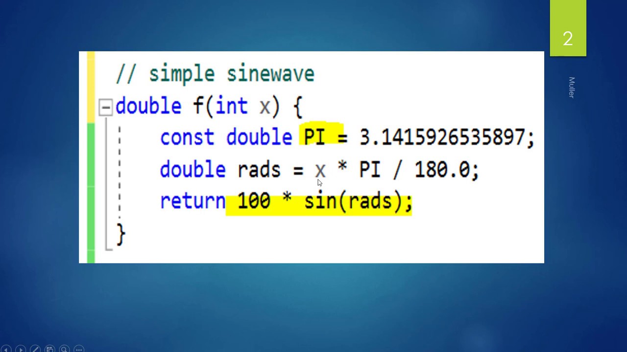


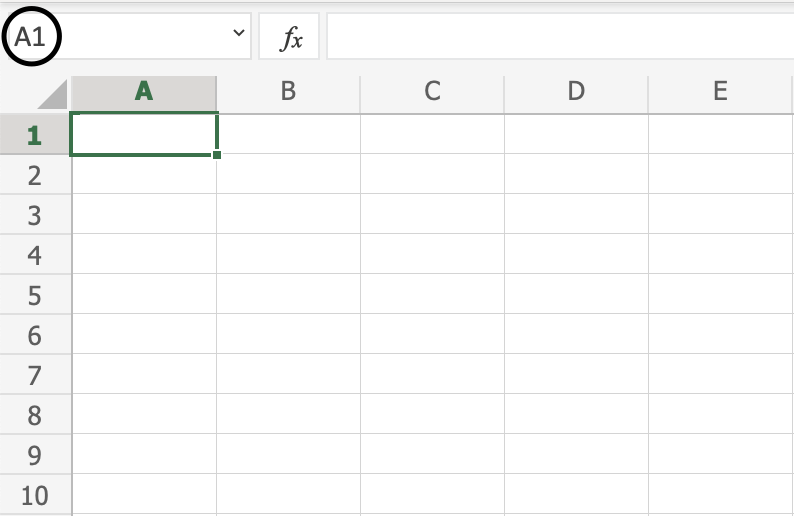
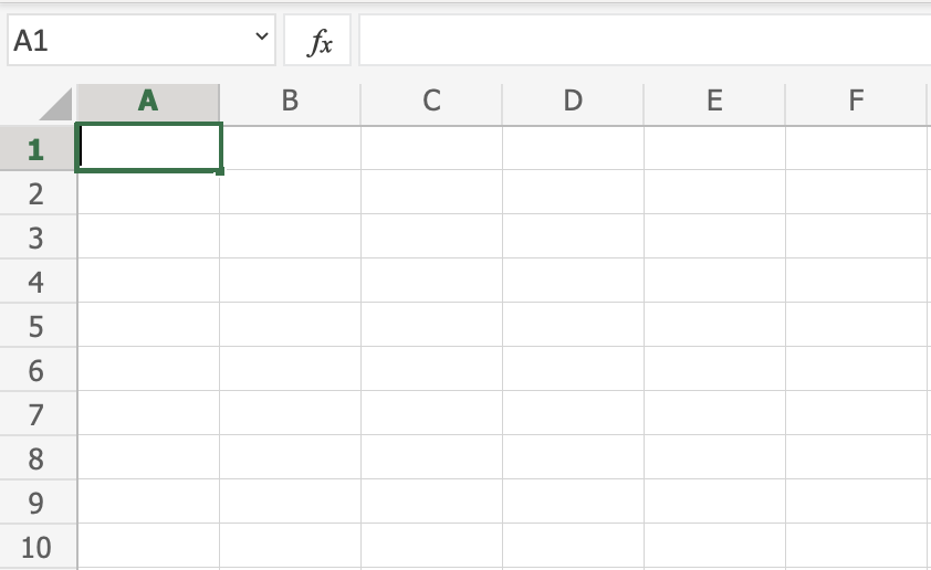
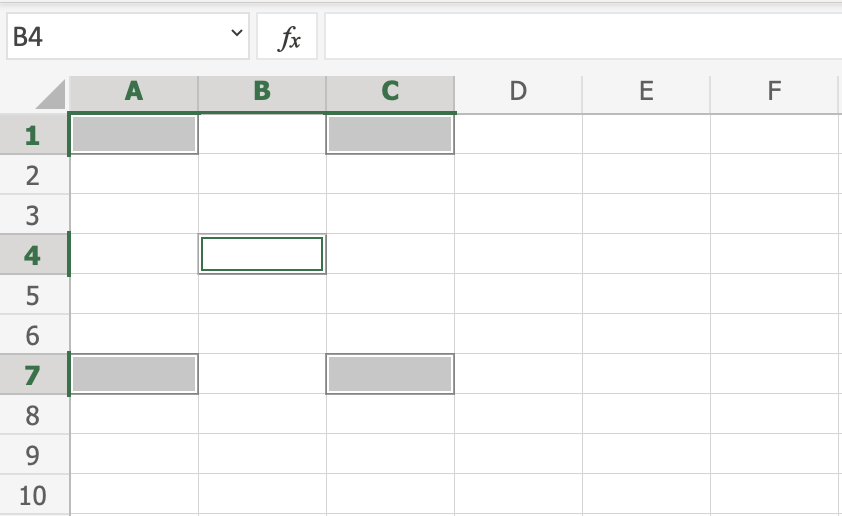
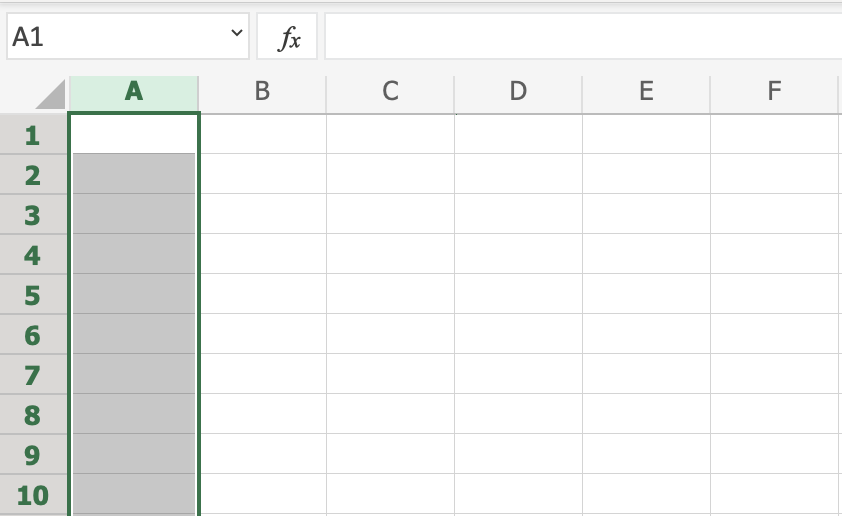
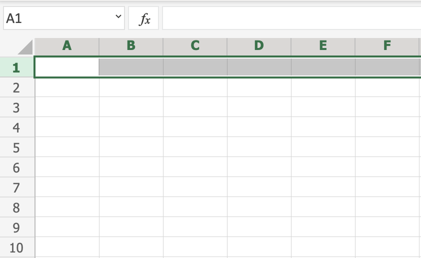
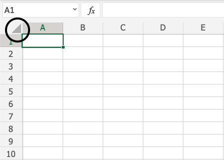
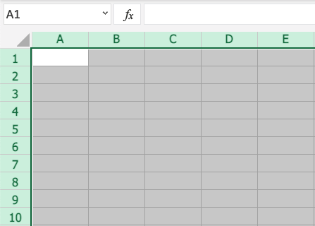
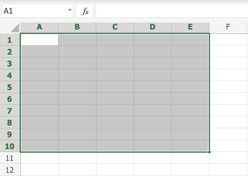
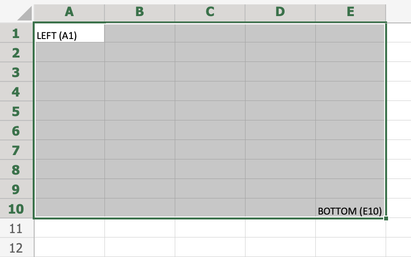
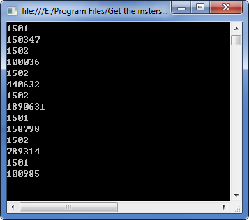
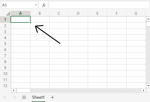
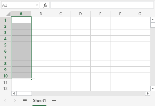
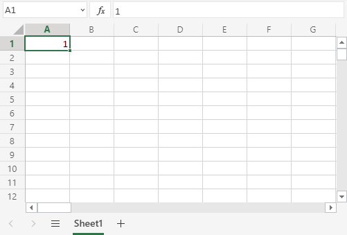
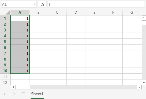
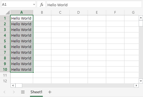
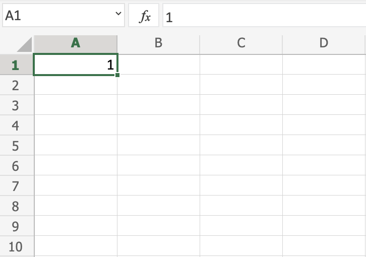
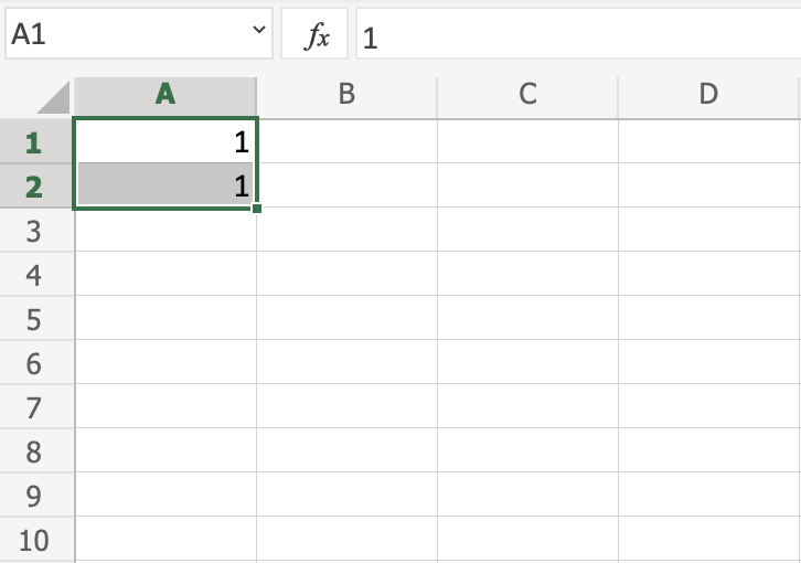
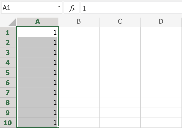
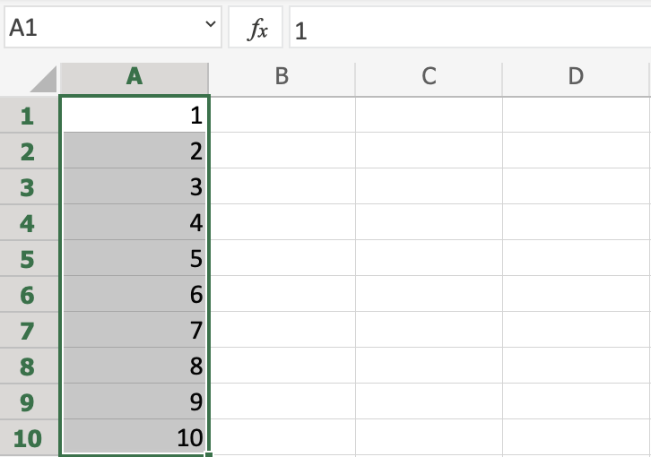
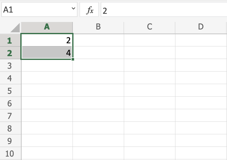
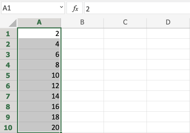
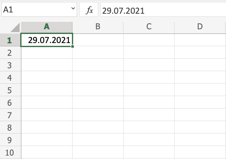
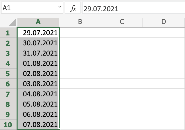
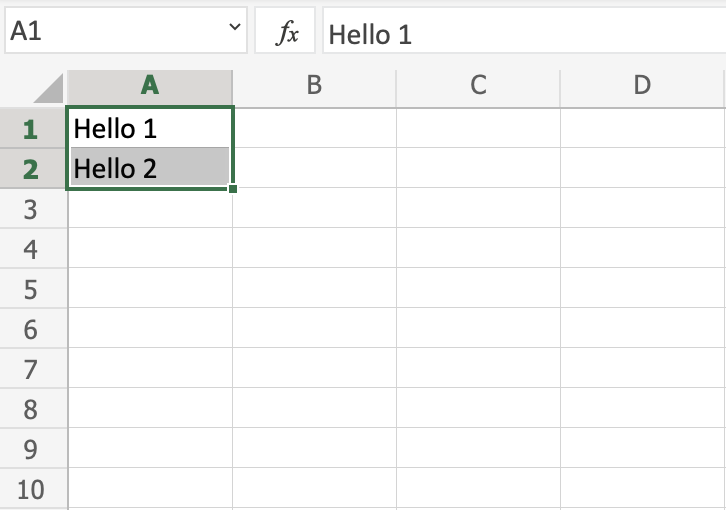
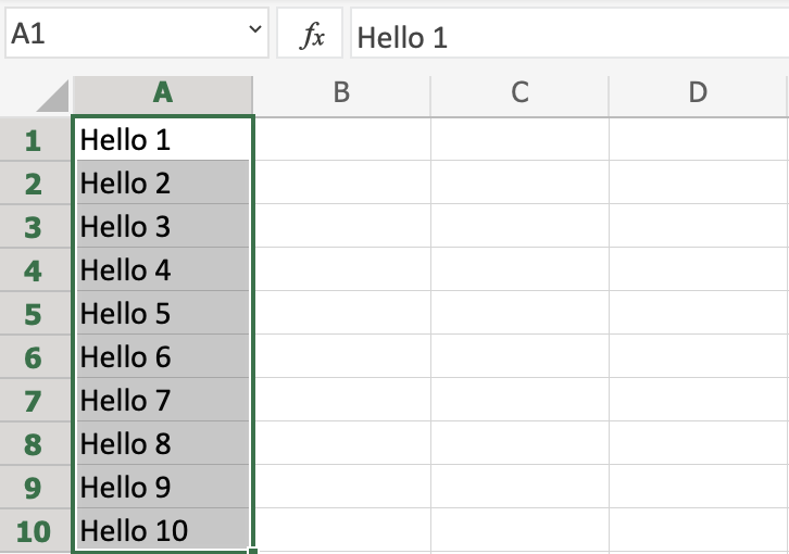
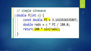
.png)


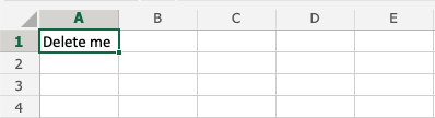
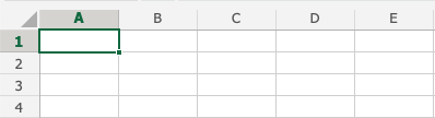
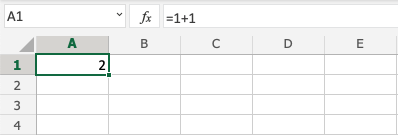
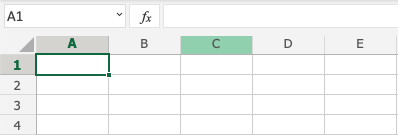
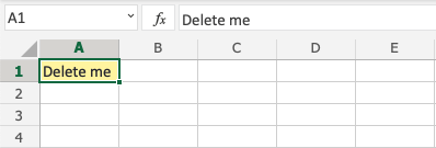
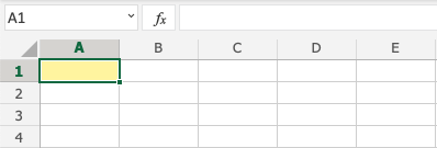
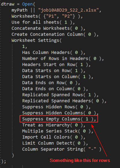
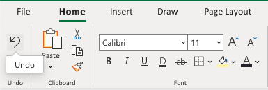
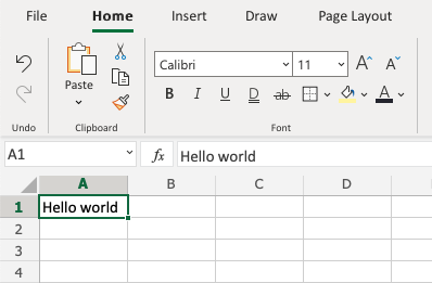
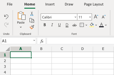
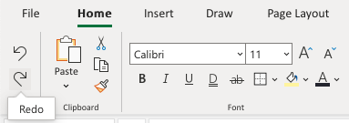


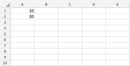
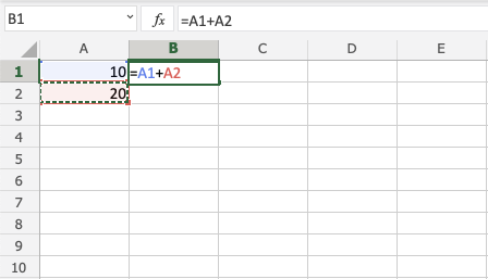
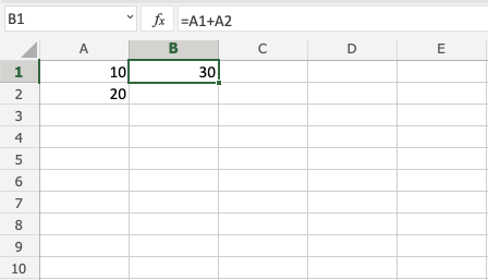
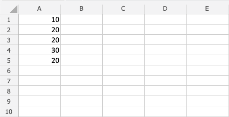
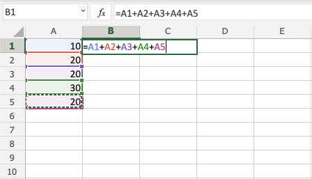
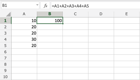
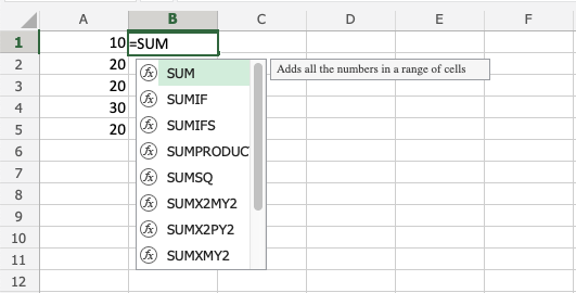
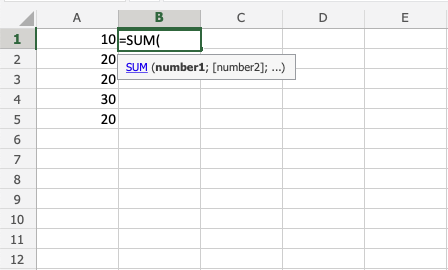
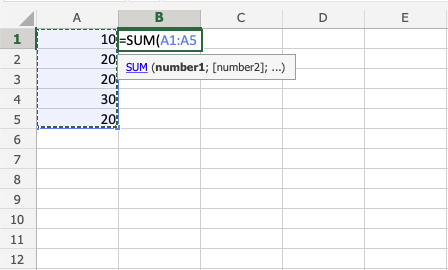
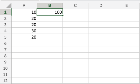
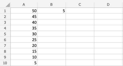

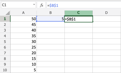

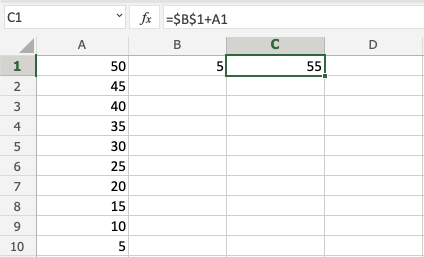

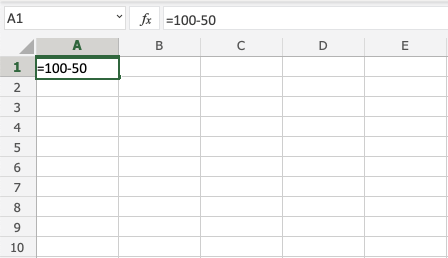
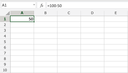

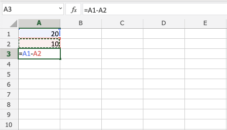
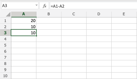
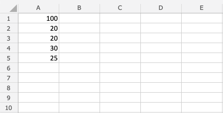
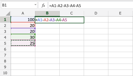
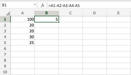


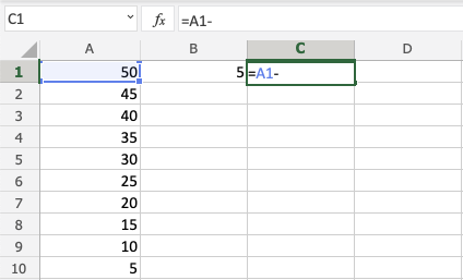
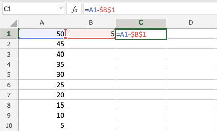

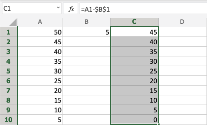
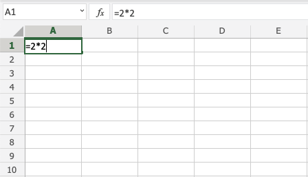
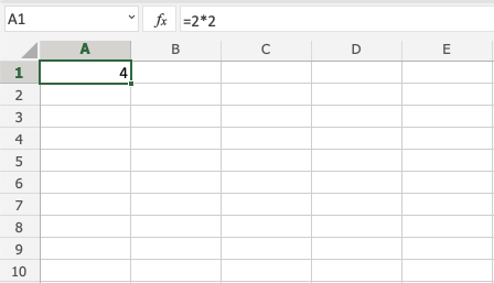

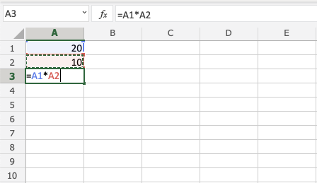
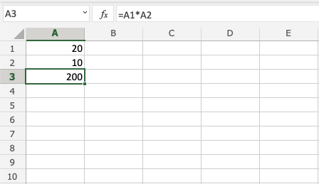
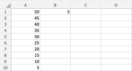
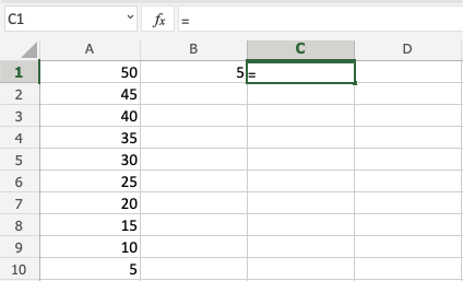
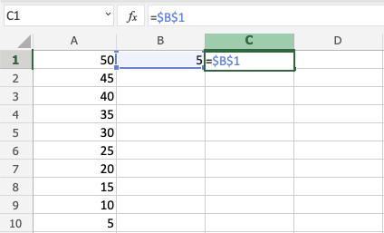
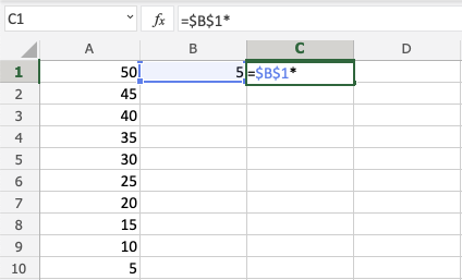
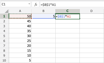
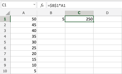

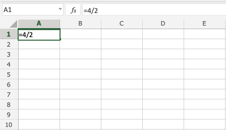
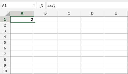
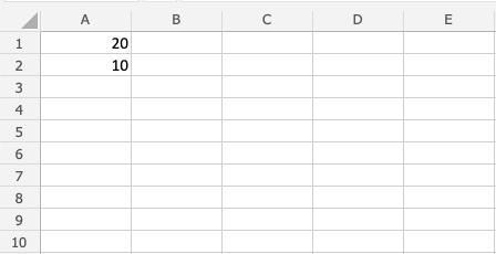
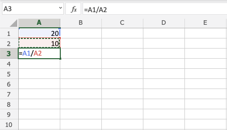
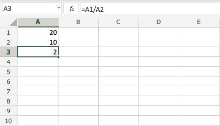


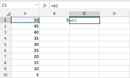
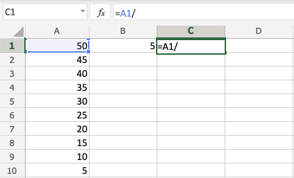
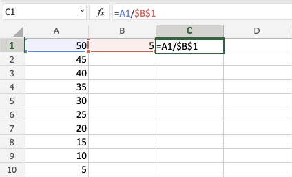


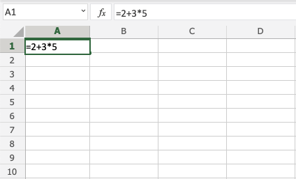


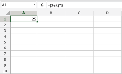
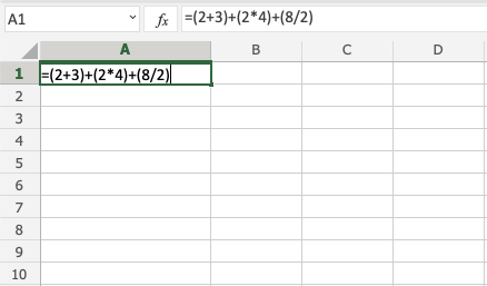
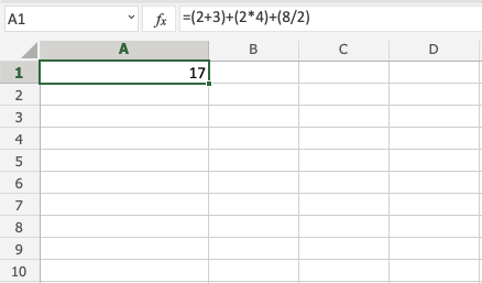
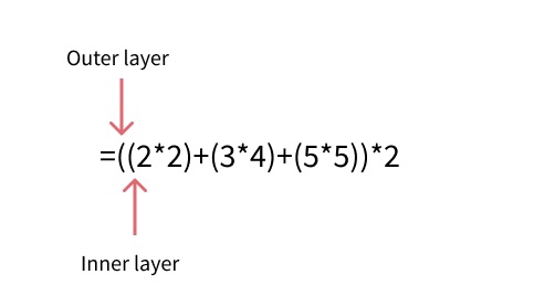


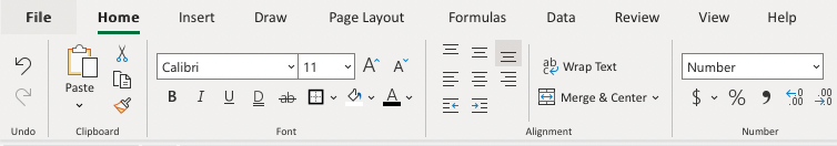
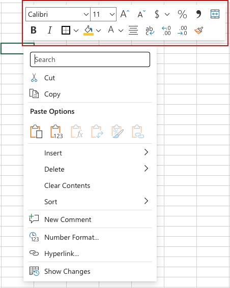
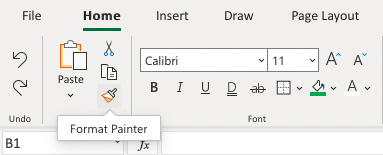
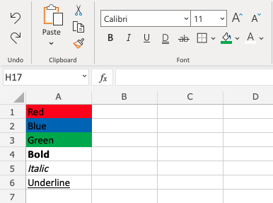
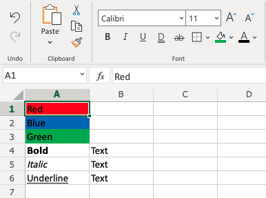
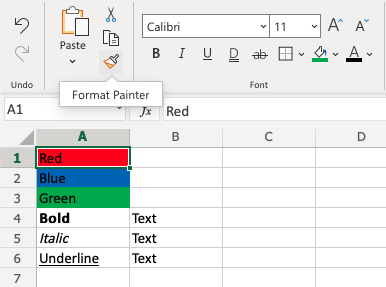

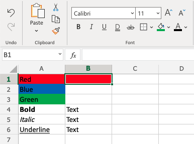

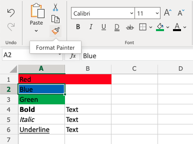
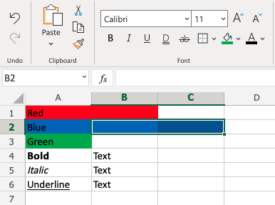
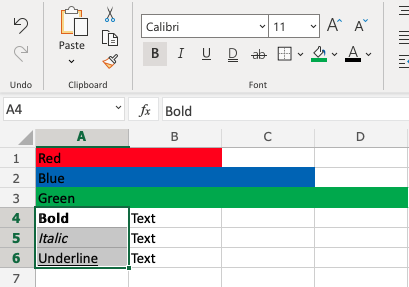
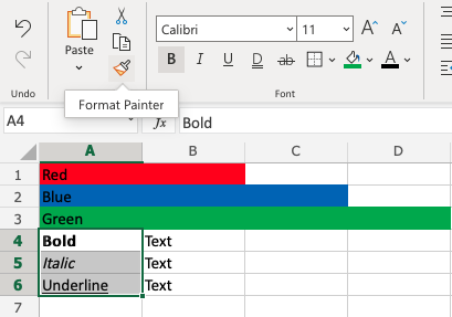

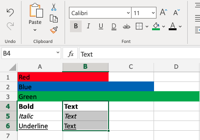
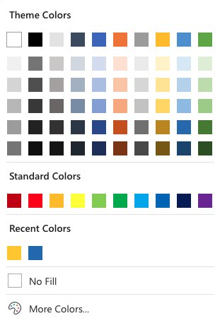
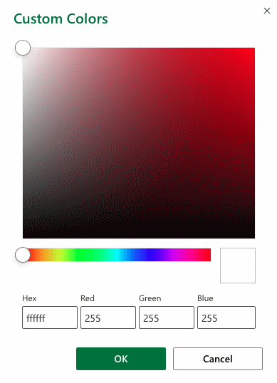
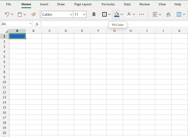
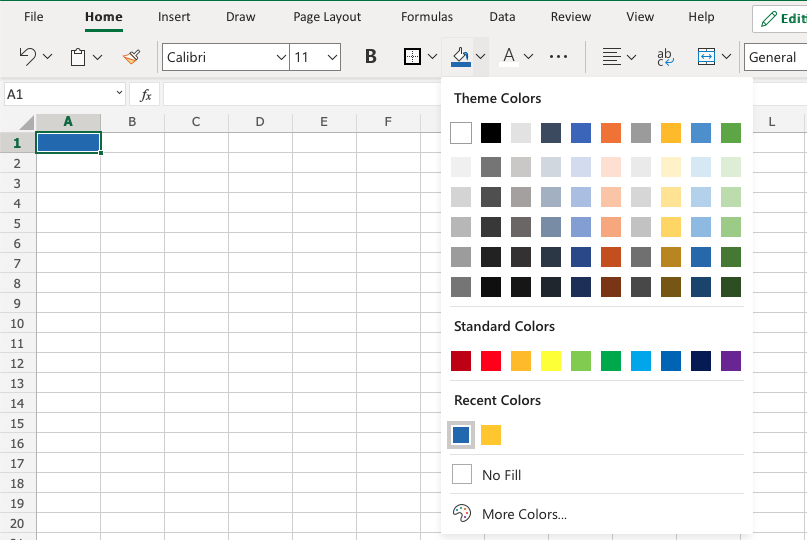
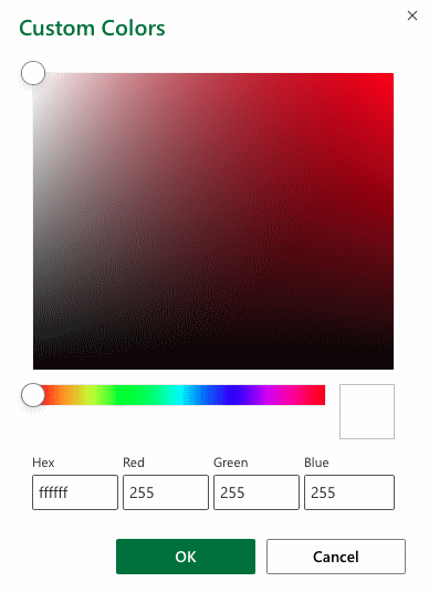
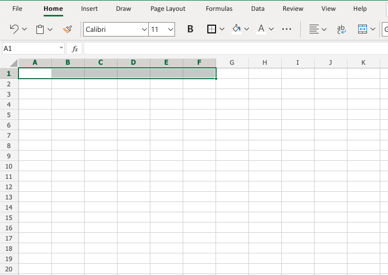
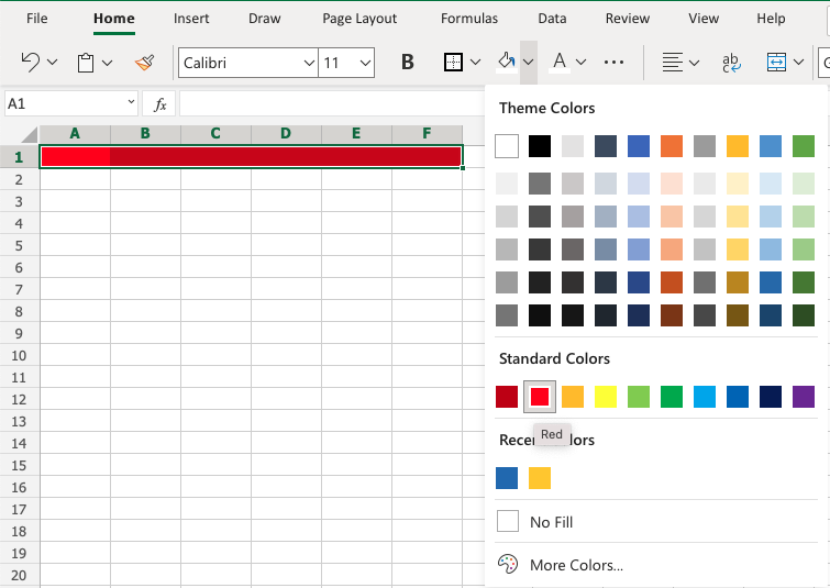

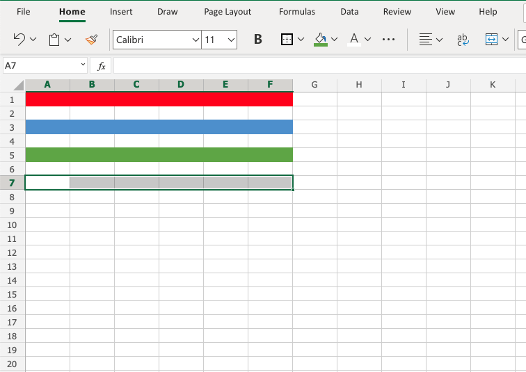
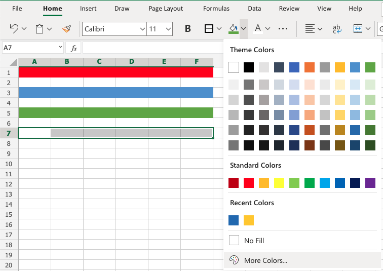
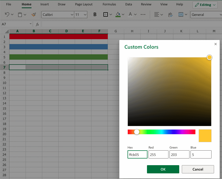

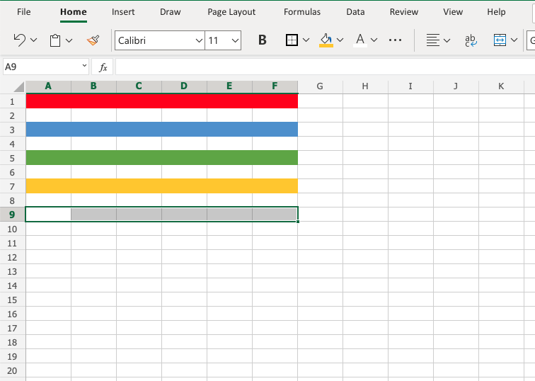
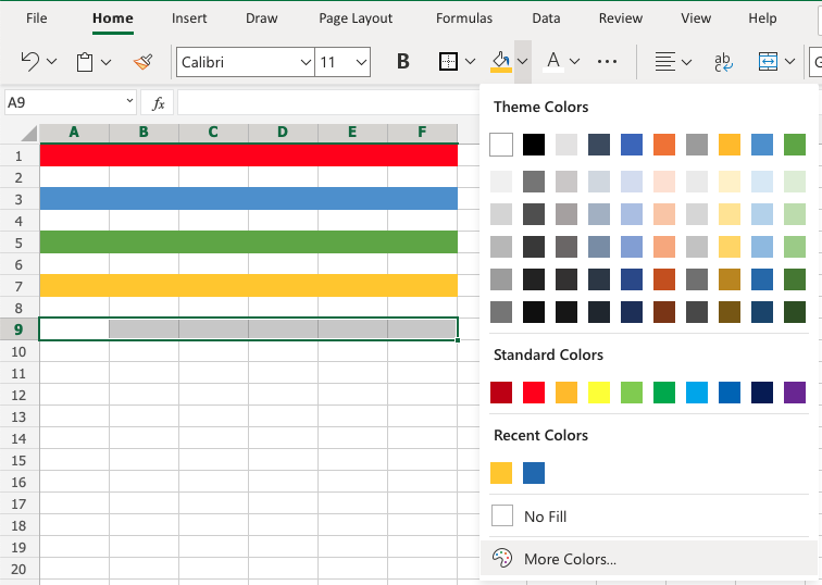

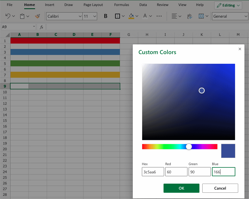
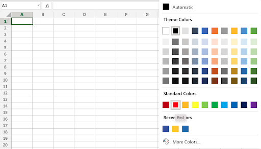
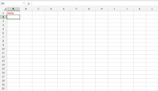
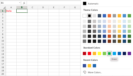
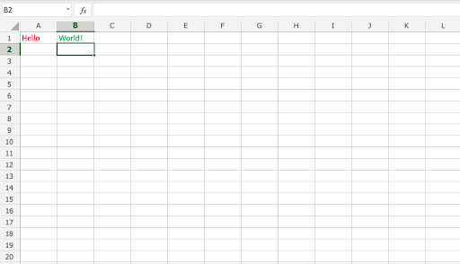
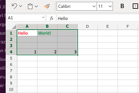
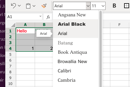
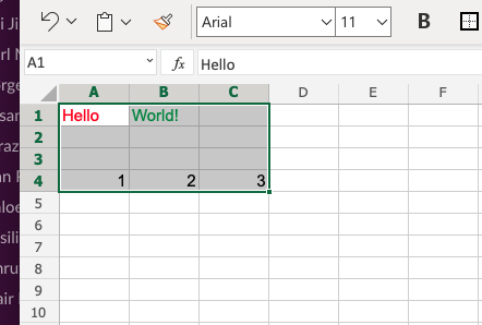
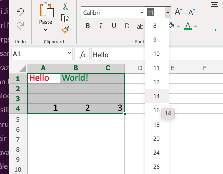
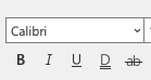
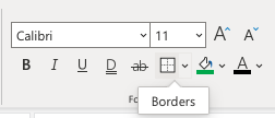
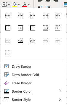
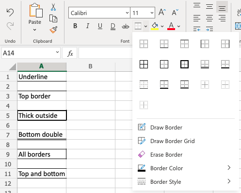
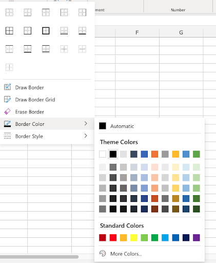

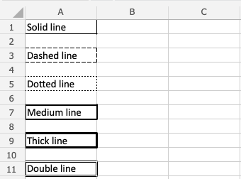
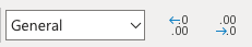
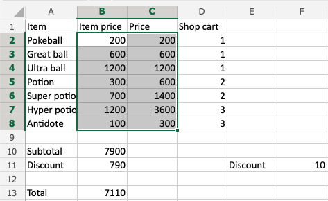
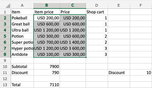
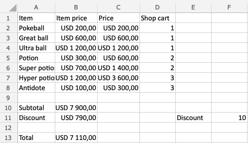
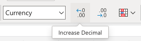
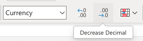
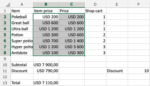
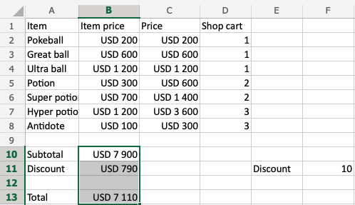
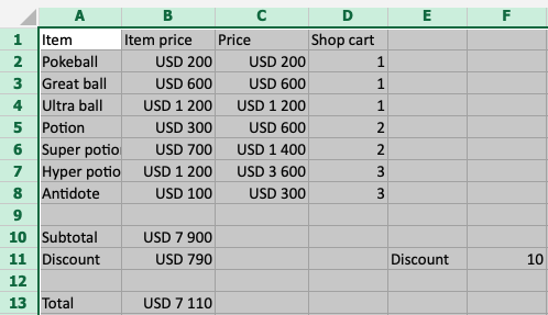

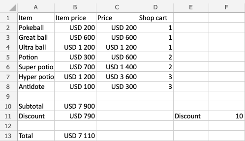
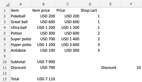
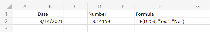
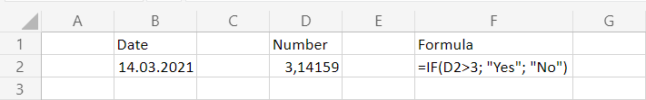
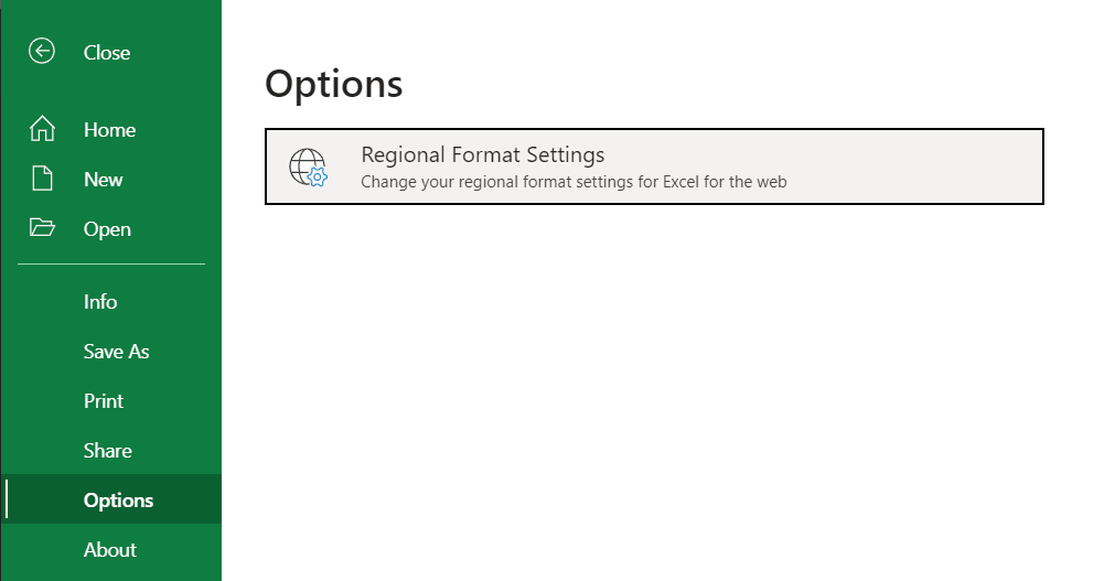
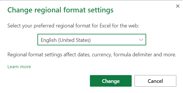


 )
)


 )
) )
)


 )
)


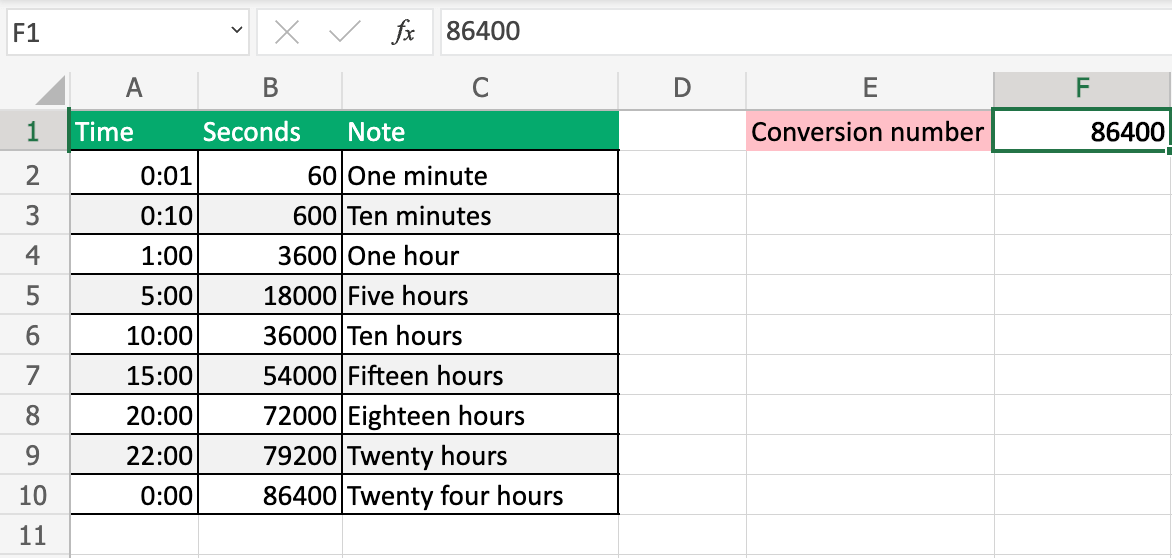


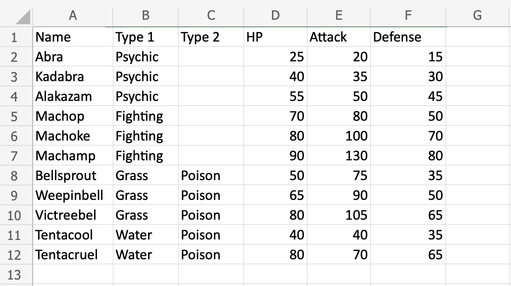
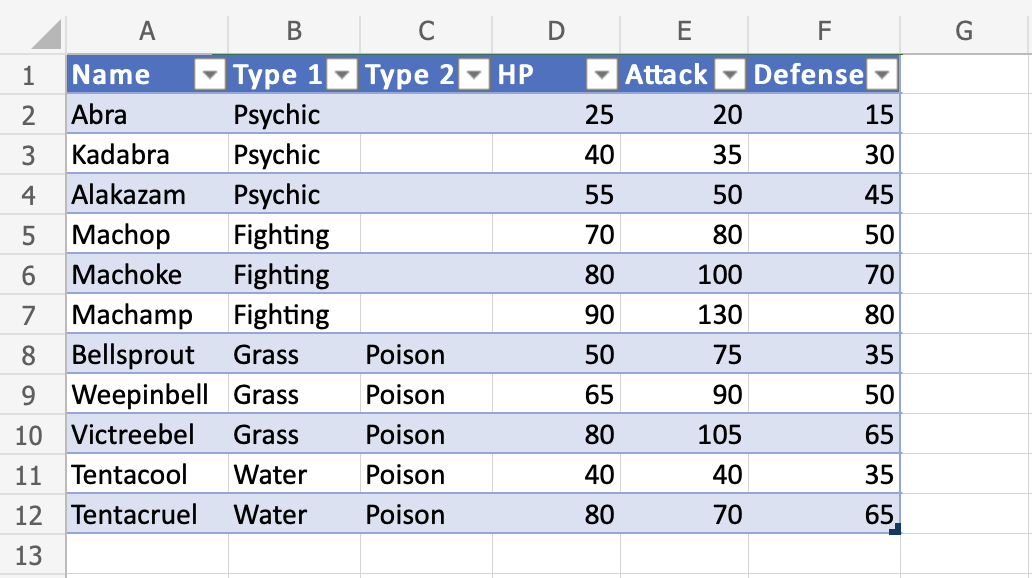
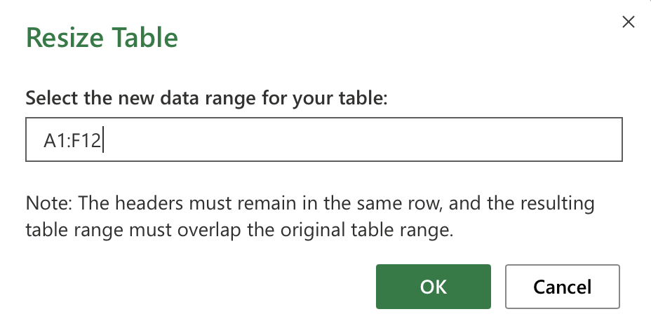
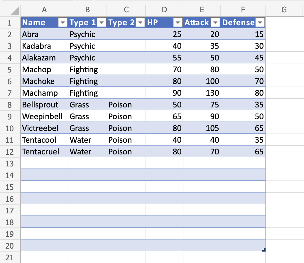
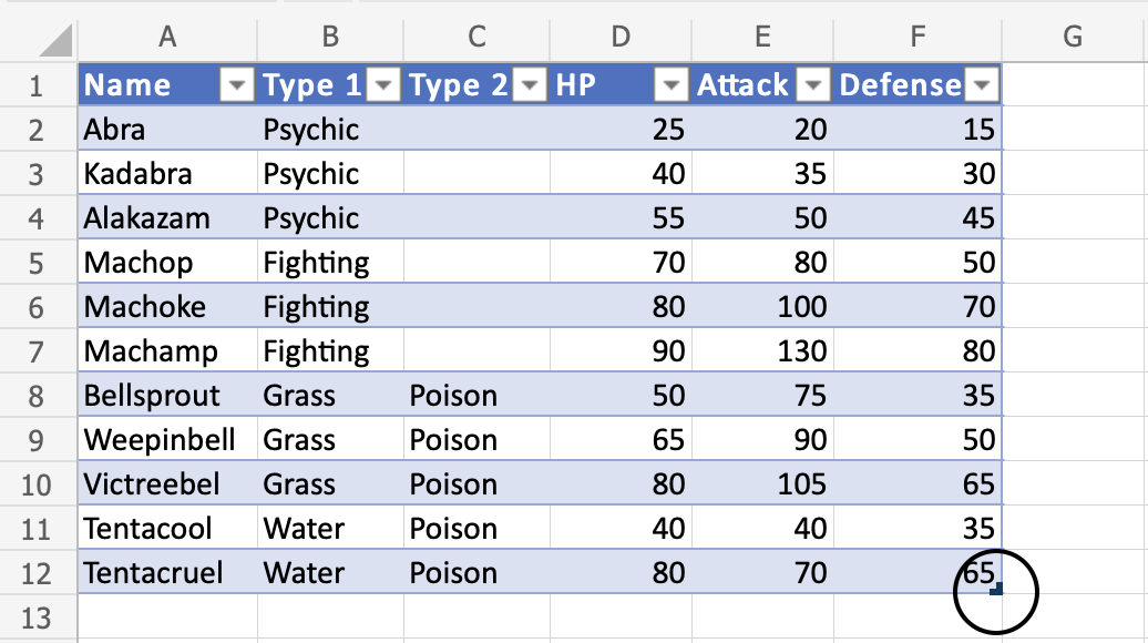
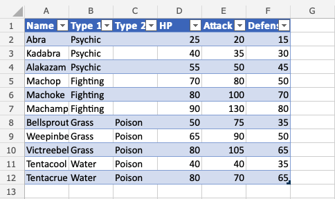
 )
)